Lasso Regression in R (Step-by-Step)

---

Lasso regression is a method we can use to fit a regression model when multicollinearity is present in the data.

In a nutshell, least squares regression tries to find coefficient estimates that minimize the sum of squared residuals (RSS):

RSS = Σ(y_i – ŷ_i)2

where:

• Σ: A greek symbol that means sum
• y_i: The actual response value for the i^th observation
• ŷ_i: The predicted response value based on the multiple linear regression model

Conversely, lasso regression seeks to minimize the following:

RSS + λΣ|β_j|

where j ranges from 1 to p predictor variables and λ ≥ 0.

This second term in the equation is known as a shrinkage penalty. In lasso regression, we select a value for λ that produces the lowest possible test MSE (mean squared error).

This tutorial provides a step-by-step example of how to perform lasso regression in R.

Step 1: Load the Data

For this example, we’ll use the R built-in dataset called mtcars. We’ll use hp as the response variable and the following variables as the predictors:

• mpg
• wt
• drat
• qsec

To perform lasso regression, we’ll use functions from the glmnet package. This package requires the response variable to be a vector and the set of predictor variables to be of the class data.matrix.

The following code shows how to define our data:

#define response variable
y #define matrix of predictor variables
x 

Step 2: Fit the Lasso Regression Model

Next, we’ll use the glmnet() function to fit the lasso regression model and specify alpha=1.

Note that setting alpha equal to 0 is equivalent to using ridge regression and setting alpha to some value between 0 and 1 is equivalent to using an elastic net. 

To determine what value to use for lambda, we’ll perform k-fold cross-validation and identify the lambda value that produces the lowest test mean squared error (MSE).

Note that the function cv.glmnet() automatically performs k-fold cross validation using k = 10 folds.

library(glmnet)

#perform k-fold cross-validation to find optimal lambda value
cv_model glmnet(x, y, alpha = 1)

#find optimal lambda value that minimizes test MSE
best_lambda lambda.min
best_lambda

[1] 5.616345

#produce plot of test MSE by lambda value
plot(cv_model) 

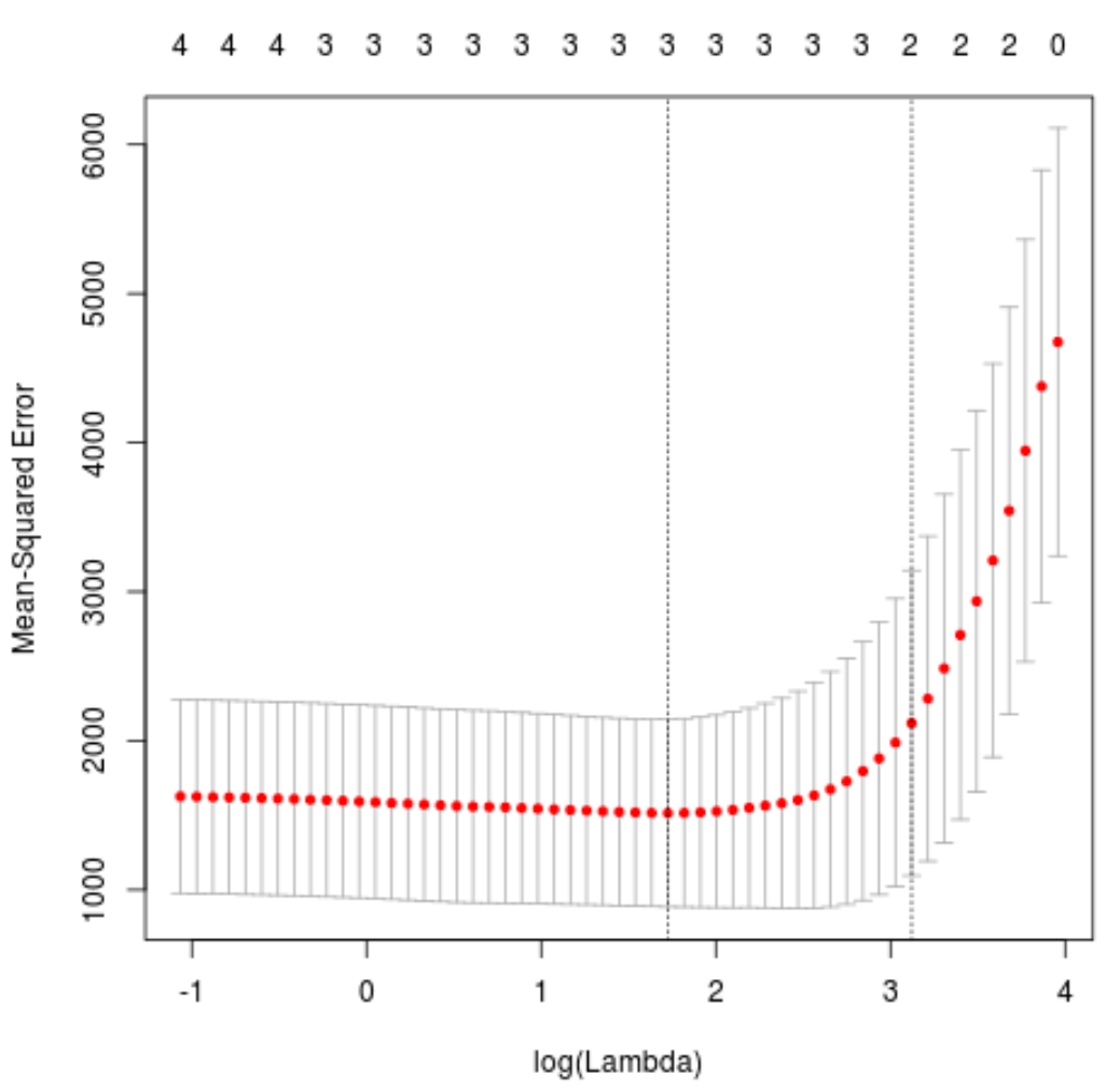
The lambda value that minimizes the test MSE turns out to be 5.616345.

Step 3: Analyze Final Model

Lastly, we can analyze the final model produced by the optimal lambda value.

We can use the following code to obtain the coefficient estimates for this model:

#find coefficients of best model
best_model 1, lambda = best_lambda)
coef(best_model)

5 x 1 sparse Matrix of class "dgCMatrix"
                   s0
(Intercept) 484.20742
mpg          -2.95796
wt           21.37988
drat          .      
qsec        -19.43425

No coefficient is shown for the predictor drat because the lasso regression shrunk the coefficient all the way to zero. This means it was completely dropped from the model because it wasn’t influential enough.

Note that this is a key difference between ridge regression and lasso regression. Ridge regression shrinks all coefficients towards zero, but lasso regression has the potential to remove predictors from the model by shrinking the coefficients completely to zero.

We can also use the final lasso regression model to make predictions on new observations. For example, suppose we have a new car with the following attributes:

• mpg: 24
• wt: 2.5
• drat: 3.5
• qsec: 18.5

The following code shows how to use the fitted lasso regression model to predict the value for hp of this new observation:

#define new observation
new = matrix(c(24, 2.5, 3.5, 18.5), nrow=1, ncol=4) 

#use lasso regression model to predict response value
predict(best_model, s = best_lambda, newx = new)

[1,] 109.0842

Based on the input values, the model predicts this car to have an hp value of 109.0842.

Lastly, we can calculate the R-squared of the model on the training data:

#use fitted best model to make predictions
y_predicted predict(best_model, s = best_lambda, newx = x)

#find SST and SSE
sst sum((y - mean(y))^2)
sse sum((y_predicted - y)^2)

#find R-Squared
rsq 

The R-squared turns out to be 0.8047064. That is, the best model was able to explain 80.47% of the variation in the response values of the training data.

You can find the complete R code used in this example here.