The central limit theorem states that the sampling distribution of a sample mean is approximately normal if the sample size is large enough, even if the population distribution is not normal.
The central limit theorem also states that the sampling distribution will have the following properties:
1. The mean of the sampling distribution will be equal to the mean of the population distribution:
x = μ
2. The variance of the sampling distribution will be equal to the variance of the population distribution divided by the sample size:
s2 = σ2 / n
Examples of the Central Limit Theorem
Here are a few examples to illustrate the central limit theorem in practice.
The Uniform Distribution
Suppose the width of a turtle’s shell follows a uniform distribution with a minimum width of 2 inches and a maximum width of 6 inches. That is, if we randomly selected a turtle and measured the width of its shell, it’s equally likely to be any width between 2 and 6 inches.
If we made a histogram to represent the distribution of turtle shell widths, it would look like this:
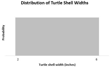
The mean of a uniform distribution is μ = (b+a) / 2 where b is the largest possible value and a is the smallest possible value. In this case, it’s (6+2) / 2 = 4.
The variance of a uniform distribution is σ2 = (b-a)2 / 12. In this case, it’s (6-2)2 / 12 = 1.33
Taking random samples of 2 from the uniform distribution
Now, imagine that we take a random sample of 2 turtles from this population and measure the width of each turtles shell. Suppose the first turtle’s shell has a width of 3 inches and the second has a width of 6 inches. The mean width for this sample of 2 turtles is 4.5 inches.
Then, imagine that we take another random sample of 2 turtles from this population and again measure the width of each turtles shell. Suppose the first turtle’s shell has a width of 2.5 inches and the second also has a width of 2.5 inches. The mean width for this sample of 2 turtles is 2.5 inches.
Imagine that we just keep taking random samples of 2 turtles over and over again and keep finding the mean shell width each time.
If we made a histogram to represent the mean shell width of all these samples of 2 turtles, it would look like this:
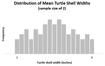
This is known as the sampling distribution for the sample mean because it shows the distribution of sample means.
The mean of this sampling distribution is x = μ = 4
The variance of this sampling distribution is s2 = σ2 / n = 1.33 / 2 = .665
Taking random samples of 5 from the uniform distribution
Now, imagine that we repeated the same experiment, but this time we take random samples of 5 turtles over and over again and find the mean shell width each time.
If we made a histogram to represent the mean shell width of all these samples of 5 turtles, it would look like this:
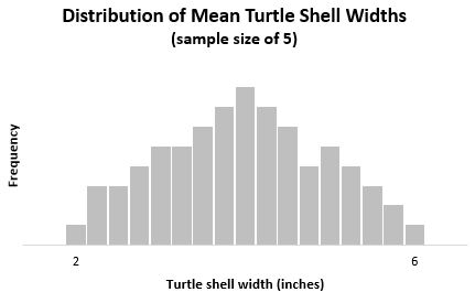
Notice how this distribution has more of a “bell” shape that resembles the normal distribution. This is because when we take samples of 5, the variance among our sample means is much lower, so we’re less likely to obtain samples where the mean is close to 2 inches or close to 6 inches and more likely to obtain samples where the mean is closer to the true population mean of 4 inches.
The mean of this sampling distribution is x = μ = 4
The variance of this sampling distribution is s2 = σ2 / n = 1.33 / 5 = .266
Taking random samples of 30 from the uniform distribution
Now, imagine that we repeated the same experiment, but this time we take random samples of 30 turtles over and over again and find the mean shell width each time.
If we made a histogram to represent the mean shell width of all these samples of 30 turtles, it would look like this:
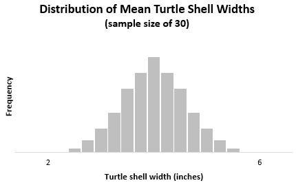
Notice how this sampling distribution has even more of a bell shape and is much narrower than the previous two distributions.
The mean of this sampling distribution is x = μ = 4
The variance of this sampling distribution is s2 = σ2 / n = 1.33 / 30 = .044
The Chi-Square Distribution
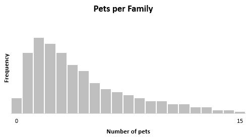
Suppose the number of pets per family in a certain city follows a chi-square distribution with three degrees of freedom. If we made a histogram to represent the distribution of pets per family, it would look like this:
The mean of a chi-square distribution is simply the number of degrees of freedom (df). In this case, μ = 3.
The variance of a chi-square distribution is 2 * df. In this case, σ2 = 2 * 3 = 6.
Taking random samples of 2
Imagine that we take a random sample of 2 families from this population and count the number of pets in each family. Suppose the first family has 4 pets and the second family has 1 pet. The mean number of pets for this sample of 2 families is 2.5.
Then, imagine that we take another random sample of 2 families from this population and again count the number of pets in each family. Suppose the first family has 6 pets and the second family has 4 pets. The mean number of pets for this sample of 2 families is 5.
Imagine that we just keep taking random samples of 2 families over and over again and keep finding the mean number of pets each time.
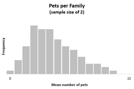
If we made a histogram to represent the mean number of pets of all these samples of 2 families, it would look like this:
The mean of this sampling distribution is x = μ = 3
The variance of this sampling distribution is s2 = σ2 / n = 6 / 2 = 3
Taking random samples of 10
Now, imagine that we repeated the same experiment, but this time we take random samples of 10 families over and over again and find the mean number of pets per family each time.
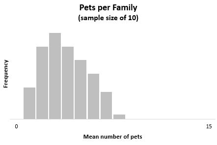
If we made a histogram to represent the mean number of pets per family in all these samples of 10 families, it would look like this:
The mean of this sampling distribution is x = μ = 3
The variance of this sampling distribution is s2 = σ2 / n = 6 / 10 = 0.6
Taking random samples of 30
Now, imagine that we repeated the same experiment, but this time we take random samples of 30 families over and over again and find the mean number of pets per family each time.
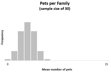
If we made a histogram to represent the mean number of pets per family in all these samples of 30 families, it would look like this:
The mean of this sampling distribution is x = μ = 3
The variance of this sampling distribution is s2 = σ2 / n = 6 / 30 = 0.2
Summary
Here are the key takeaways from these two examples:
- The sampling distribution of a sample mean is approximately normal if the sample size is large enough, even if the population distribution is not normal. In the two examples above, neither the uniform distribution nor the chi-square distribution were normal (they didn’t have a “bell” shape at all), yet when we took a large enough sample size, the distribution of the sample mean turned out to be normal.
- The larger the sample size, the smaller the variance of the sample mean.
Defining “Large Enough”
Recall that the central limit theorem states that the sampling distribution of a sample mean is approximately normal if the sample size is “large enough”, even if the population distribution is not normal.
There is no exact definition for how large a sample size needs to be in order for the central limit theorem to apply, but in general it depends on the skewness of the population distribution that the sample comes from:
- If the population distribution is symmetric, sometimes a sample size as small as 15 is sufficient.
- If the population distribution is skewed, generally a sample size of at least 30 is needed.
- If the population distribution is extremely skewed, then a sample size of 40 or higher may be necessary.
Check out this tutorial on The Large Sample Condition for more information on this topic.
