When we have a dataset with one predictor variable and one response variable, we often use simple linear regression to quantify the relationship between the two variables.
However, simple linear regression (SLR) assumes that the relationship between the predictor and response variable is linear. Written in mathematical notation, SLR assumes that the relationship takes the form:
Y = β0 + β1X + ε
But in practice the relationship between the two variables can actually be nonlinear and attempting to use linear regression can result in a poorly fit model.
One way to account for a nonlinear relationship between the predictor and response variable is to use polynomial regression, which takes the form:
Y = β0 + β1X + β2X2 + … + βhXh + ε
In this equation, h is referred to as the degree of the polynomial.
As we increase the value for h, the model is able to fit nonlinear relationships better, but in practice we rarely choose h to be greater than 3 or 4. Beyond this point, the model becomes too flexible and overfits the data.
Technical Notes
- Although polynomial regression can fit nonlinear data, it is still considered to be a form of linear regression because it is linear in the coefficients β1, β2, …, βh.
- Polynomial regression can be used for multiple predictor variables as well but this creates interaction terms in the model, which can make the model extremely complex if more than a few predictor variables are used.
When to Use Polynomial Regression
We use polynomial regression when the relationship between a predictor and response variable is nonlinear.
There are three common ways to detect a nonlinear relationship:
1. Create a Scatterplot.
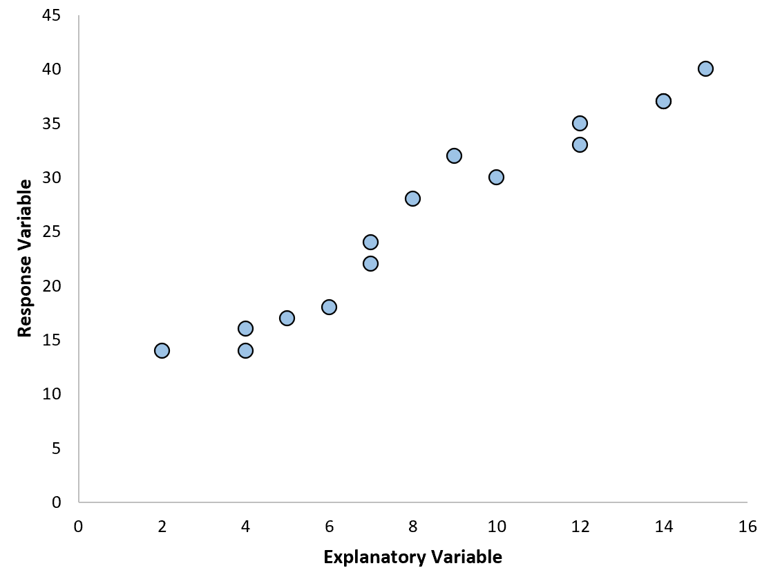
The easiest way to detect a nonlinear relationship is to create a scatterplot of the response vs. predictor variable.
For example, if we create the following scatterplot then we can see that the relationship between the two variables is roughly linear, thus simple linear regression would likely perform fine on this data.
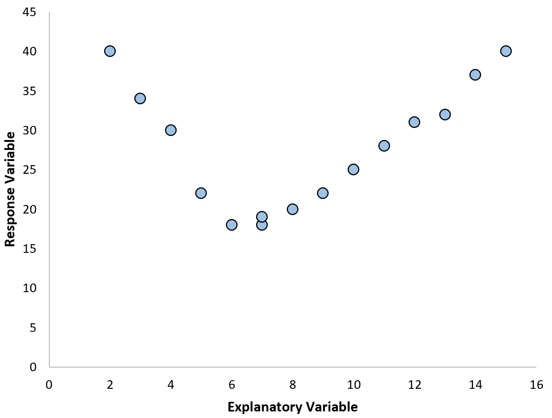
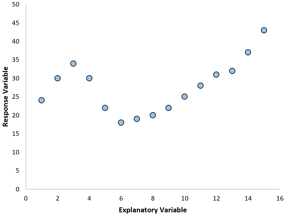
However, if our scatterplot looks like one of the following plots then we could see that the relationship is nonlinear and thus polynomial regression would be a good idea:
2. Create a residuals vs. fitted plot.
Another way to detect nonlinearity is to fit a simple linear regression model to the data and then produce a residuals vs. fitted values plot.
If the residuals of the plot are roughly evenly distributed around zero with no clear pattern, then simple linear regression is likely sufficient.
However, if the residuals display a nonlinear pattern in the plot then this is a sign that the relationship between the predictor and the response is likely nonlinear.
3. Calculate the R2 of the model.
The R2 value of a regression model tells you the percentage of the variation in the response variable that can be explained by the predictor variable(s).
If you fit a simple linear regression model to a dataset and the R2 value of the model is quite low, this could be an indication that the relationship between the predictor and response variable is more complex than just a simple linear relationship.
This could be a sign that you may need to try polynomial regression instead.
Related: What is a Good R-squared Value?
How to Choose the Degree of the Polynomial
A polynomial regression model takes the following form:
Y = β0 + β1X + β2X2 + … + βhXh + ε
In this equation, h is the degree of the polynomial.
But how do we choose a value for h?
In practice, we fit several different models with different values of h and perform k-fold cross-validation to determine which model produces the lowest test mean squared error (MSE).
For example, we may fit the following models to a given dataset:
- Y = β0 + β1X
- Y = β0 + β1X + β2X2
- Y = β0 + β1X + β2X2 + β3X3
- Y = β0 + β1X + β2X2 + β3X3 + β4X4
We can then use k-fold cross-validation to calculate the test MSE of each model, which will tell us how well each model performs on data it hasn’t seen before.
The Bias-Variance Tradeoff of Polynomial Regression
There exists a bias-variance tradeoff when using polynomial regression. As we increase the degree of the polynomial, the bias decreases (as the model becomes more flexible) but the variance increases.
As with all machine learning models, we must find an optimal tradeoff between bias and variance.
In most cases it helps to increase the degree of the polynomial to an extent, but beyond a certain value the model begins to fit the noise of the data and the test MSE begins to decrease.
To ensure that we fit a model that is flexible but not too flexible, we use k-fold cross-validation to find the model that produces the lowest test MSE.
How to Perform Polynomial Regression
The following tutorials provide examples of how to perform polynomial regression in different softwares:
How to Perform Polynomial Regression in Excel
How to Perform Polynomial Regression in R
How to Perform Polynomial Regression in Python