Multiple linear regression is a method you can use to understand the relationship between several explanatory variables and a response variable.
This tutorial explains how to perform multiple linear regression in Stata.
Example: Multiple Linear Regression in Stata
Suppose we want to know if miles per gallon and weight impact the price of a car. To test this, we can perform a multiple linear regression using miles per gallon and weight as the two explanatory variables and price as the response variable.
Perform the following steps in Stata to conduct a multiple linear regression using the dataset called auto, which contains data on 74 different cars.
Step 1: Load the data.
Load the data by typing the following into the Command box:
use http://www.stata-press.com/data/r13/auto
Step 2: Get a summary of the data.
Gain a quick understanding of the data you’re working with by typing the following into the Command box:
summarize
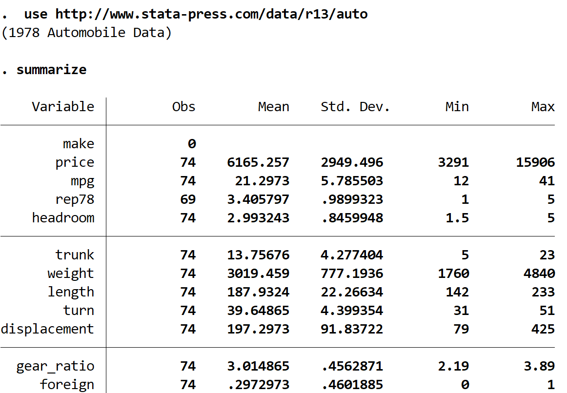
We can see that there are 12 different variables in the dataset, but the only ones we care about are mpg, weight, and price.
We can see the following basic summary statistics about these three variables:
price | mean = $6,165, min = $3,291, max $15,906
mpg | mean = 21.29, min = 12, max = 41
weight | mean = 3,019 pounds, min = 1,760 pounds, max = 4,840 pounds
Step 3: Perform multiple linear regression.
Type the following into the Command box to perform a multiple linear regression using mpg and weight as explanatory variables and price as a response variable.
regress price mpg weight
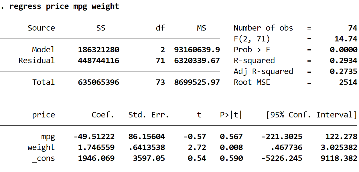
Here is how to interpret the most interesting numbers in the output:
Prob > F: 0.000. This is the p-value for the overall regression. Since this value is less than 0.05, this indicates that the combined explanatory variables of mpg and weight have a statistically significant relationship with the response variable price.
R-squared: 0.2934. This is the proportion of the variance in the response variable that can be explained by the explanatory variables. In this example, 29.34% of the variation in price can be explained by mpg and weight.
Coef (mpg): -49.512. This tells us the average change in price that is associated with a one unit increase in the mpg, assuming weight is held constant. In this example, each one unit increase in mpg is associated with an average decrease of about $49.51 in price, assuming weight is held constant.
For example, suppose cars A and B both weigh 2,000 pounds. If car A gets 20 mpg and car B only gets 19 mpg, we would expect the price of car A to be $49.51 less than the price of car B.
P>|t| (mpg): 0.567. This is the p-value associated with the test statistic for mpg. Since this value is not less than 0.05, we don’t have evidence to say that mpg has a statistically significant relationship with price.
Coef (weight): 1.746. This tells us the average change in price that is associated with a one unit increase in weight, assuming mpg is held constant. In this example, each one unit increase in weight is associated with an average increase of about $1.74 in price, assuming mpg is held constant.
For example, suppose cars A and B both get 20 mpg. If car A weighs one pound more than car B, then car A is expected to cost $1.74 more.
P>|t| (weight): 0.008. This is the p-value associated with the test statistic for weight. Since this value is less than 0.05, we have sufficient evidence to say that weight has a statistically significant relationship with price.
Coef (_cons): 1946.069. This tells us the average price of a car when both mpg and weight are zero. In this example, the average price is $1,946 when both weight and mpg are zero. This doesn’t actually make much sense to interpret since the weight and mpg of a car can’t be zero, but the number 1946.069 is needed to form a regression equation.
Step 4: Report the results.
Lastly, we want to report the results of our multiple linear regression. Here is an example of how to do so:
Multiple linear regression was performed to quantify the relationship between the weight and mpg of a car and its price. A sample of 74 cars was used in the analysis.
Results showed that there was a statistically significant relationship between weight and price (t = 2.72, p = .008), but there was not a statistically significant relationship between mpg and price (and mpg (t = -.57, p = 0.567).