An ANOVA is a statistical test that is used to determine whether or not there is a statistically significant difference between the means of three or more independent groups.
The hypotheses used in an ANOVA are as follows:
The null hypothesis (H0): µ1 = µ2 = µ3 = … = µk (the means are equal for each group)
The alternative hypothesis: (Ha): at least one of the means is different from the others
If the p-value from the ANOVA is less than the significance level, we can reject the null hypothesis and conclude that we have sufficient evidence to say that at least one of the means of the groups is different from the others.
However, this doesn’t tell us which groups are different from each other. It simply tells us that not all of the group means are equal.
In order to find out exactly which groups are different from each other, we must conduct a post hoc test (also known as a multiple comparison test), which will allow us to explore the difference between multiple group means while also controlling for the family-wise error rate.
Technical Note: It’s important to note that we only need to conduct a post hoc test when the p-value for the ANOVA is statistically significant. If the p-value is not statistically significant, this indicates that the means for all of the groups are not different from each other, so there is no need to conduct a post hoc test to find out which groups are different from each other.
The Family-Wise Error Rate
As mentioned before, post hoc tests allow us to test for difference between multiple group means while also controlling for the family-wise error rate.
In a hypothesis test, there is always a type I error rate, which is defined by our significance level (alpha) and tells us the probability of rejecting a null hypothesis that is actually true. In other words, it’s the probability of getting a “false positive”, i.e. when we claim there is a statistically significant difference among groups, but there actually isn’t.
When we perform one hypothesis test, the type I error rate is equal to the significance level, which is commonly chosen to be 0.01, 0.05, or 0.10. However, when we conduct multiple hypothesis tests at once, the probability of getting a false positive increases.
For example, imagine that we roll a 20-sided dice. The probability that the dice lands on a “1” is just 5%. But if we roll two dice at once, the probability that one of the dice will land on a “1” increases to 9.75%. If we roll five dice at once, the probability increases to 22.6%.
The more dice we roll, the higher the probability that one of the dice will land on a “1.” Similarly, if we conduct several hypothesis tests at once using a significance level of .05, the probability that we get a false positive increases to beyond just 0.05.
Multiple Comparisons in ANOVA
When we conduct an ANOVA, there are often three or more groups that we are comparing to one another. Thus, when we conduct a post hoc test to explore the difference between the group means, there are several pairwise comparisons we want to explore.
For example, suppose we have four groups: A, B, C, and D. This means there are a total of six pairwise comparisons we want to look at with a post hoc test:
A – B (the difference between the group A mean and the group B mean)
A – C
A – D
B – C
B – D
C – D
If we have more than four groups, the number of pairwise comparisons we will want to look at will only increase even more. The following table illustrates how many pairwise comparisons are associated with each number of groups along with the family-wise error rate:
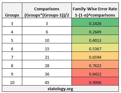
Notice that the family-wise error rate increases rapidly as the number of groups (and consequently the number of pairwise comparisons) increases. In fact, once we reach six groups, the probability of us getting a false positive is actually above 50%!
This means we would have serious doubts about our results if we were to make this many pairwise comparisons, knowing that our family-wise error rate was so high.
Fortunately, post hoc tests provide us with a way to make multiple comparisons between groups while controlling the family-wise error rate.
Example: One-Way ANOVA with Post Hoc Tests
The following example illustrates how to perform a one-way ANOVA with post hoc tests.
Note: This example uses the programming language R, but you don’t need to know R to understand the results of the test or the big takeaways.
First, we’ll create a dataset that contains four groups (A, B, C, D) with 20 observations per group:
#make this example reproducible
set.seed(1)

#load tidyr library to convert data from wide to long format
library(tidyr)

#create wide dataset
data #convert to long dataset for ANOVA
data_long #view first six lines of dataset
head(data_long)

#  group   amount
#1     A 2.796526
#2     A 3.116372
#3     A 3.718560
#4     A 4.724623
#5     A 2.605046
#6     A 4.695169
Next, we’ll fit a one-way ANOVA to the dataset:
#fit anova model
anova_model #view summary of anova model
summary(anova_model)

#            Df Sum Sq Mean Sq F value   Pr(>F)
#group        3  25.37   8.458   17.66 8.53e-09 ***
#Residuals   76  36.39   0.479
From the ANOVA table output, we see that the F-statistic is 17.66 and the corresponding p-value is extremely small.
This means we have sufficient evidence to reject the null hypothesis that all of the group means are equal. Next, we can use a post hoc test to find which group means are different from each other.
We will walk through examples of the following post hoc tests:
Tukey’s Test – useful when you want to make every possible pairwise comparison
Holm’s Method – a slightly more conservative test compared to Tukey’s Test
Dunnett’s Correction – useful when you want to compare every group mean to a control mean, and you’re not interested in comparing the treatment means with one another.
Tukey’s Test
We can perform Tukey’s Test for multiple comparisons by using the built-in R function TukeyHSD() as follows:
#perform Tukey's Test for multiple comparisons
TukeyHSD(anova_model, conf.level=.95)

#  Tukey multiple comparisons of means
#    95% family-wise confidence level
#
#Fit: aov(formula = amount ~ group, data = data_long)
#
#$group
#         diff          lwr       upr     p adj
#B-A 0.2822630 -0.292540425 0.8570664 0.5721402
#C-A 0.8561388  0.281335427 1.4309423 0.0011117
#D-A 1.4676027  0.892799258 2.0424061 0.0000000
#C-B 0.5738759 -0.000927561 1.1486793 0.0505270
#D-B 1.1853397  0.610536271 1.7601431 0.0000041
#D-C 0.6114638  0.036660419 1.1862672 0.0326371
Notice that we specified our confidence level to be 95%, which means we want our family-wise error rate to be .05. R gives us two metrics to compare each pairwise difference:
- Confidence interval for the mean difference (given by the values of lwr and upr)
- Adjusted p-value for the mean difference
Both the confidence interval and the p-value will lead to the same conclusion.
For example, the 95% confidence interval for the mean difference between group C and group A is (0.2813, 1.4309), and since this interval doesn’t contain zero we know that the difference between these two group means is statistically significant. In particular, we know that the difference is positive, since the lower bound of the confidence interval is greater than zero.
Likewise, the p-value for the mean difference between group C and group A is 0.0011, which is less than our significance level of 0.05, so this also indicates that the difference between these two group means is statistically significant.
We can also visualize the 95% confidence intervals that result from the Tukey Test by using the plot() function in R:
plot(TukeyHSD(anova_model, conf.level=.95))
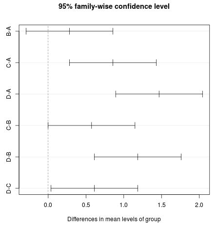
If the interval contains zero, then we know that the difference in group means is not statistically significant. In the example above, the differences for B-A and C-B are not statistically significant, but the differences for the other four pairwise comparisons are statistically significant.
Holm’s Method
Another post hoc test we can perform is holm’s method. This is generally viewed as a more conservative test compared to Tukey’s Test.
We can use the following code in R to perform holm’s method for multiple pairwise comparisons:
#perform holm's method for multiple comparisons
pairwise.t.test(data_long$amount, data_long$group, p.adjust="holm")
#	Pairwise comparisons using t tests with pooled SD
#
#data:  data_long$amount and data_long$group
#
#  A       B       C
#B 0.20099 -       -
#C 0.00079 0.02108 -
#D 1.9e-08 3.4e-06 0.01974
#
#P value adjustment method: holm
This test provides a grid of p-values for each pairwise comparison. For example, the p-value for the difference between the group A and group B mean is 0.20099.
If you compare the p-values of this test with the p-values from Tukey’s Test, you’ll notice that each of the pairwise comparisons lead to the same conclusion, except for the difference between group C and D. The p-value for this difference was .0505 in Tukey’s Test compared to .02108 in Holm’s Method.
Thus, using Tukey’s Test we concluded that the difference between group C and group D was not statistically significant at the .05 significance level, but using Holm’s Method we concluded that the difference between group C and group D was statistically significant.
In general, the p-values produced by Holm’s Method tend to be lower than those produced by Tukey’s Test.
Dunnett’s Correction
Yet another method we can use for multiple comparisons is Dunett’s Correction. We would use this approach when we want to compare every group mean to a control mean, and we’re not interested in comparing the treatment means with one another.
For example, using the code below we compare the group means of B, C, and D all to that of group A. So, we use group A as our control group and we aren’t interested in the differences between groups B, C, and D.
#load multcomp library necessary for using Dunnett's Correction
library(multcomp)

#convert group variable to factor
data_long$group #fit anova model
anova_model #perform comparisons
dunnet_comparison #view summary of comparisons
summary(dunnet_comparison)

#Multiple Comparisons of Means: Dunnett Contrasts
#
#Fit: aov(formula = amount ~ group, data = data_long)
#
#Linear Hypotheses:
#           Estimate Std. Error t value Pr(>|t|)
#B - A == 0   0.2823     0.2188   1.290 0.432445
#C - A == 0   0.8561     0.2188   3.912 0.000545 ***
#D - A == 0   1.4676     0.2188   6.707
From the p-values in the output we can see the following:
- The difference between the group B and group A mean is not statistically significant at a significance level of .05. The p-value for this test is 0.4324.
- The difference between the group C and group A mean is statistically significant at a significance level of .05. The p-value for this test is 0.0005.
- The difference between the group D and group A mean is statistically significant at a significance level of .05. The p-value for this test is 0.00004.
As we stated earlier, this approach treats group A as the “control” group and simply compares every other group mean to that of group A. Notice that there are no tests performed for the differences between groups B, C, and D because we aren’t interested in the differences between those groups.
A Note on Post Hoc Tests & Statistical Power
Post hoc tests do a great job of controlling the family-wise error rate, but the tradeoff is that they reduce the statistical power of the comparisons. This is because the only way to lower the family-wise error rate is to use a lower significance level for all of the individual comparisons.
For example, when we use Tukey’s Test for six pairwise comparisons and we want to maintain a family-wise error rate of .05, we must use a significance level of approximately 0.011 for each individual significance level. The more pairwise comparisons we have, the lower the significance level we must use for each individual significance level.
The problem with this is that lower significance levels correspond to lower statistical power. This means that if a difference between group means actually does exist in the population, a study with lower power is less likely to detect it.
One way to reduce the effects of this tradeoff is to simply reduce the number of pairwise comparisons we make. For example, in the previous examples we performed six pairwise comparisons for the four different groups. However, depending on the needs of your study, you may only be interested in making a few comparisons.
By making fewer comparisons, you don’t have to lower the statistical power as much.
It’s important to note that you should determine before you perform the ANOVA exactly which groups you want to make comparisons between and which post hoc test you will use to make these comparisons. Otherwise, if you simply see which post hoc test produces statistically significant results, that reduces the integrity of the study.
Conclusion
In this post, we learned the following things:
- An ANOVA is used to determine whether or not there is a statistically significant difference between the means of three or more independent groups.
- If an ANOVA produces a p-value that is less than our significance level, we can use post hoc tests to find out which group means differ from one another.
- Post hoc tests allow us to control the family-wise error rate while performing multiple pairwise comparisons.
- The tradeoff of controlling the family-wise error rate is lower statistical power. We can reduce the effects of lower statistical power by making fewer pairwise comparisons.
- You should determine beforehand which groups you’d like to make pairwise comparisons on and which post hoc test you will use to do so.