You can use the following basic syntax to use the SEARCH function with multiple values in Google Sheets:
=FILTER(A2:A10, SEARCH("Backup", A2:A10), SEARCH("Guard", A2:A10))
This particular example will return all cells in the range A2:A10 that contain both the string “Backup” and “Guard” somewhere in the cell.
The following example shows how to use this syntax in practice.
Example: Using SEARCH with Multiple Values in Google Sheets
Suppose we have the following dataset in Google Sheets that contains information about various basketball players:
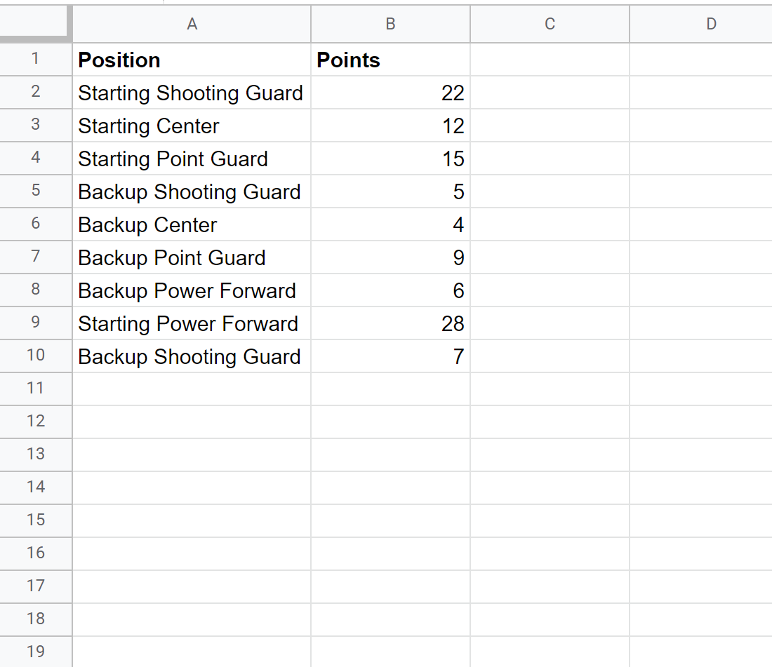
Now suppose we would like to find all cells in the Position column that contain both the word “Backup” and “Guard” somewhere in the cell.
We can type the following formula into cell D1 to find each of these cells:
=FILTER(A2:A10, SEARCH("Backup", A2:A10), SEARCH("Guard", A2:A10))
The following screenshot shows how to use this formula in practice:
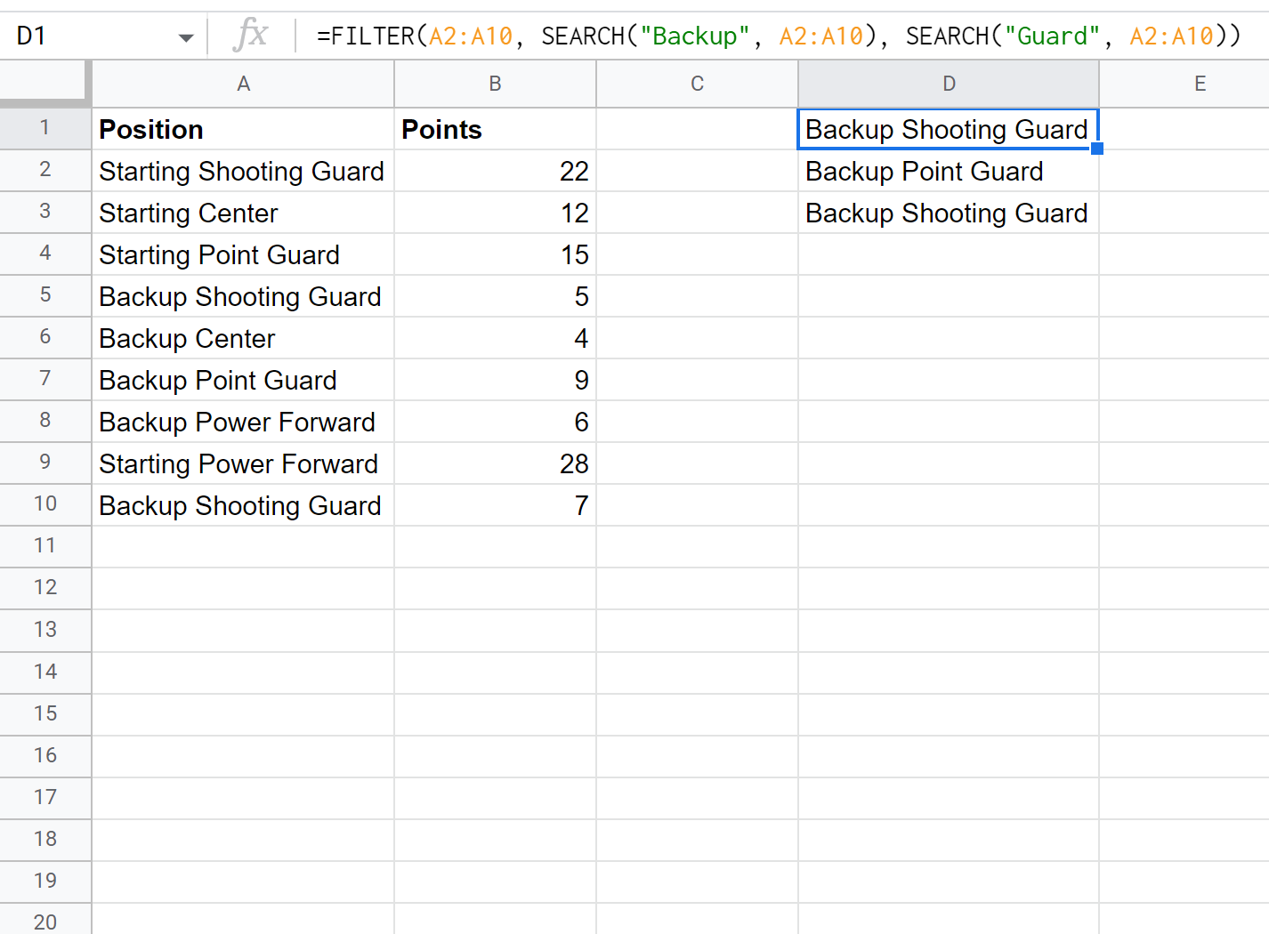
The formula correctly returns the three cells that each contain the word “Backup” and “Guard” somewhere in the cell.
If you’d like to return the values in the points column for each of these players as well, simply change the filter range from A2:A10 to A2:B10 as follows:
=FILTER(A2:B10, SEARCH("Backup", A2:A10), SEARCH("Guard", A2:A10))
The following screenshot shows how to use this formula in practice:
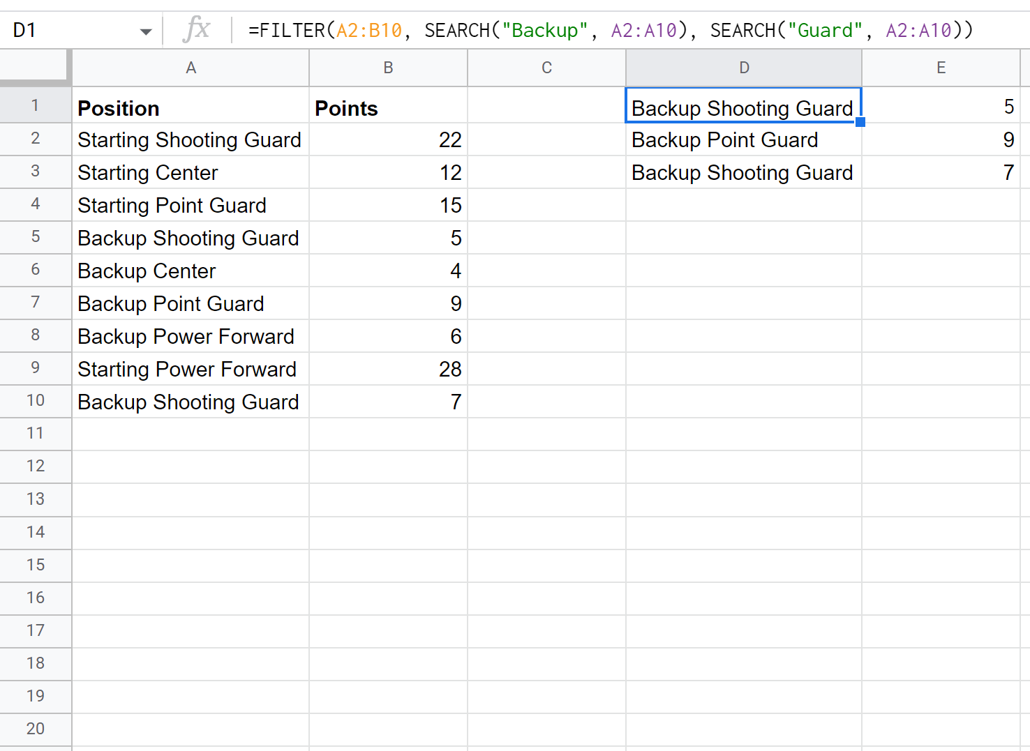
The formula now returns each cell that contains “Backup” and “Guard” in the cell along with the corresponding points values for each of these players.
Additional Resources
The following tutorials explain how to perform other common operations in Google Sheets:
How to Perform a Reverse VLOOKUP in Google Sheets
How to Use a Case Sensitive VLOOKUP in Google Sheets
How to Use INDEX MATCH with Multiple Criteria in Google Sheets