Ridge regression is a method we can use to fit a regression model when multicollinearity is present in the data.
In a nutshell, least squares regression tries to find coefficient estimates that minimize the sum of squared residuals (RSS):
RSS = Σ(yi – ŷi)2
where:
- Σ: A greek symbol that means sum
- yi: The actual response value for the ith observation
- ŷi: The predicted response value based on the multiple linear regression model
Conversely, ridge regression seeks to minimize the following:
RSS + λΣβj2
where j ranges from 1 to p predictor variables and λ ≥ 0.
This second term in the equation is known as a shrinkage penalty. In ridge regression, we select a value for λ that produces the lowest possible test MSE (mean squared error).
This tutorial provides a step-by-step example of how to perform ridge regression in R.
Step 1: Load the Data
For this example, we’ll use the R built-in dataset called mtcars. We’ll use hp as the response variable and the following variables as the predictors:
- mpg
- wt
- drat
- qsec
To perform ridge regression, we’ll use functions from the glmnet package. This package requires the response variable to be a vector and the set of predictor variables to be of the class data.matrix.
The following code shows how to define our data:
#define response variable
y #define matrix of predictor variables
x
Step 2: Fit the Ridge Regression Model
Next, we’ll use the glmnet() function to fit the ridge regression model and specify alpha=0.
Note that setting alpha equal to 1 is equivalent to using Lasso Regression and setting alpha to some value between 0 and 1 is equivalent to using an elastic net.
Also note that ridge regression requires the data to be standardized such that each predictor variable has a mean of 0 and a standard deviation of 1.
Fortunately glmnet() automatically performs this standardization for you. If you happened to already standardize the variables, you can specify standardize=False.
library(glmnet)

#fit ridge regression model
model 0)

#view summary of model
summary(model)

          Length Class     Mode
a0        100    -none-    numeric
beta      400    dgCMatrix S4
df        100    -none-    numeric
dim         2    -none-    numeric
lambda    100    -none-    numeric
dev.ratio 100    -none-    numeric
nulldev     1    -none-    numeric
npasses     1    -none-    numeric
jerr        1    -none-    numeric
offset      1    -none-    logical
call        4    -none-    call
nobs        1    -none-    numeric
Step 3: Choose an Optimal Value for Lambda
Next, we’ll identify the lambda value that produces the lowest test mean squared error (MSE) by using k-fold cross-validation.
Fortunately, glmnet has the function cv.glmnet() that automatically performs k-fold cross validation using k = 10 folds.
#perform k-fold cross-validation to find optimal lambda value
cv_model glmnet(x, y, alpha = 0)

#find optimal lambda value that minimizes test MSE
best_lambda lambda.min
best_lambda

[1] 10.04567

#produce plot of test MSE by lambda value
plot(cv_model)
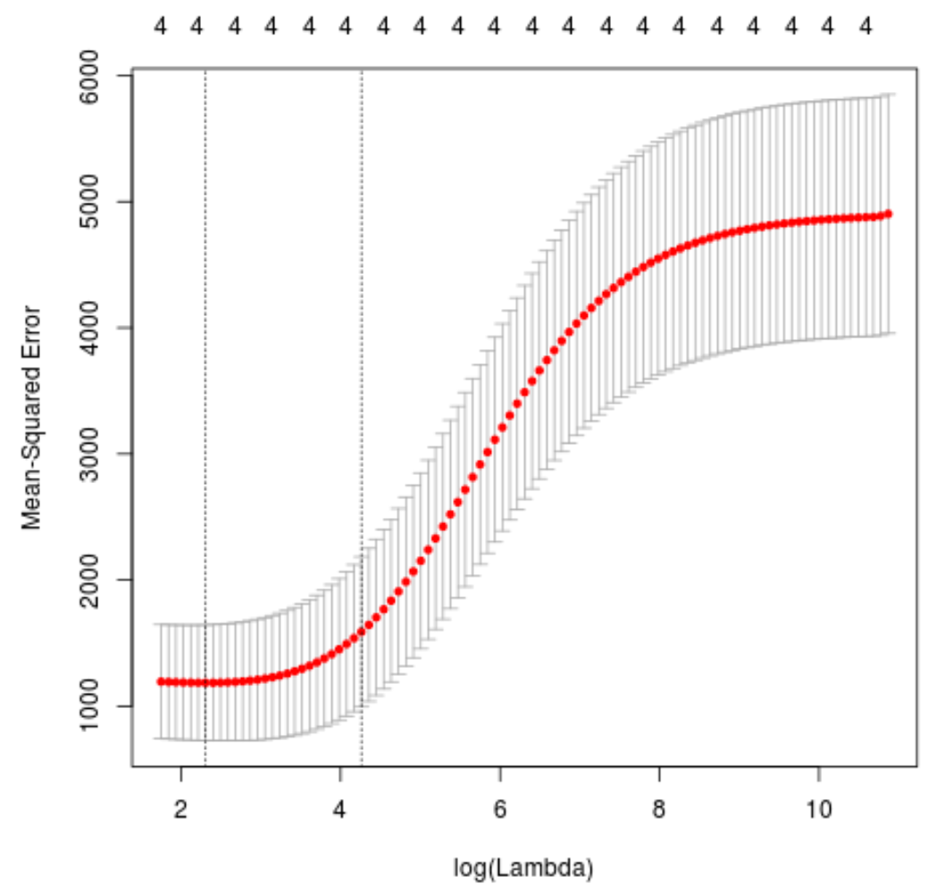
The lambda value that minimizes the test MSE turns out to be 10.04567.
Step 4: Analyze Final Model
Lastly, we can analyze the final model produced by the optimal lambda value.
We can use the following code to obtain the coefficient estimates for this model:
#find coefficients of best model
best_model 0, lambda = best_lambda)
coef(best_model)

5 x 1 sparse Matrix of class "dgCMatrix"
                    s0
(Intercept) 475.242646
mpg          -3.299732
wt           19.431238
drat         -1.222429
qsec        -17.949721
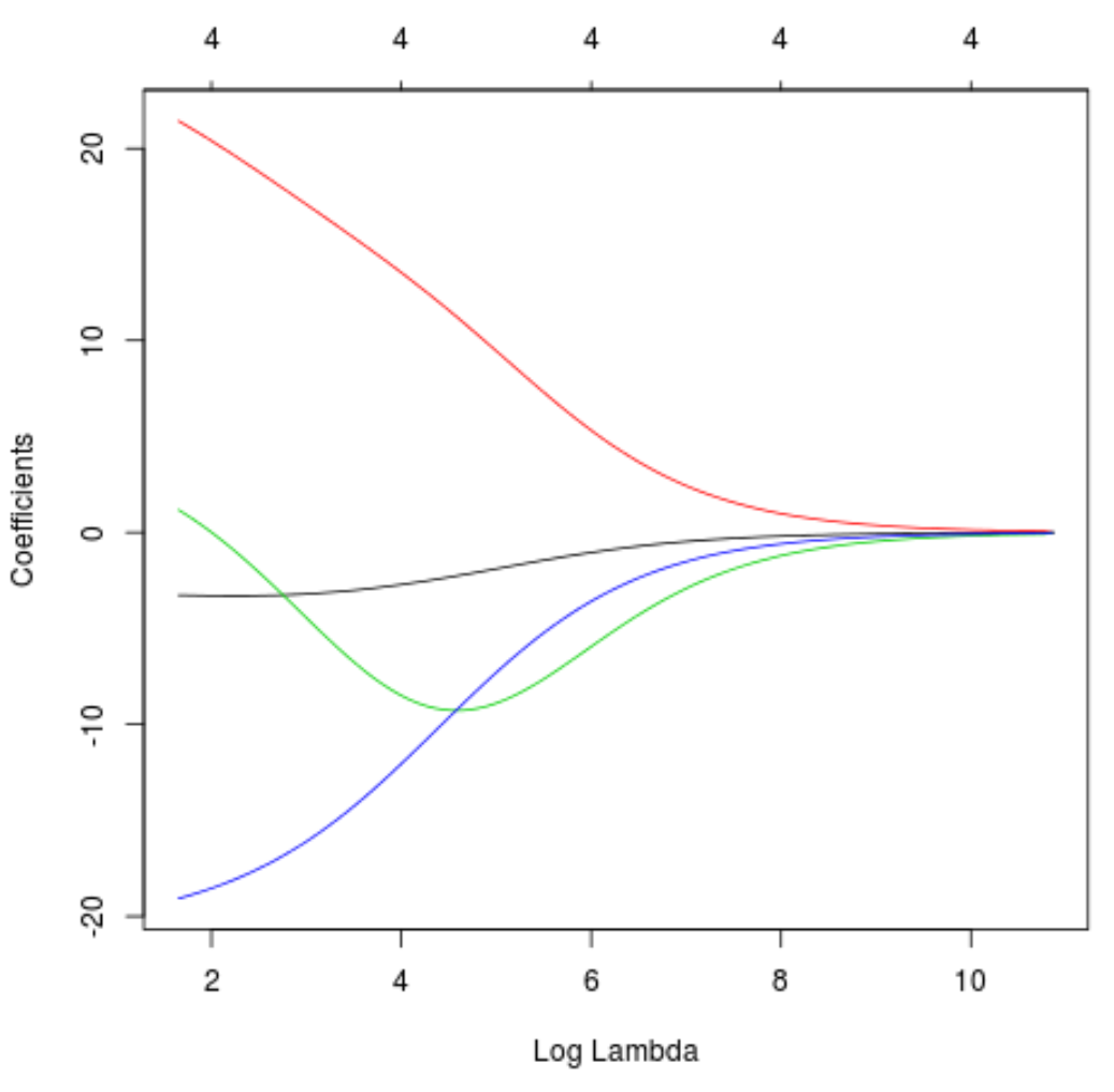
We can also produce a Trace plot to visualize how the coefficient estimates changed as a result of increasing lambda:
#produce Ridge trace plot
plot(model, xvar = "lambda")
Lastly, we can calculate the R-squared of the model on the training data:
#use fitted best model to make predictions
y_predicted predict(model, s = best_lambda, newx = x)

#find SST and SSE
sst sum((y - mean(y))^2)
sse sum((y_predicted - y)^2)

#find R-Squared
rsq
The R-squared turns out to be 0.7999513. That is, the best model was able to explain 79.99% of the variation in the response values of the training data.
You can find the complete R code used in this example here.