Simple linear regression is a statistical method you can use to understand the relationship between two variables, x and y.
One variable, x, is known as the predictor variable.
The other variable, y, is known as the response variable.
For example, suppose we have the following dataset with the weight and height of seven individuals:

Let weight be the predictor variable and let height be the response variable.
If we graph these two variables using a scatterplot, with weight on the x-axis and height on the y-axis, here’s what it would look like:

Suppose we’re interested in understanding the relationship between weight and height. From the scatterplot we can clearly see that as weight increases, height tends to increase as well, but to actually quantify this relationship between weight and height, we need to use linear regression.
Using linear regression, we can find the line that best “fits” our data. This line is known as the least squares regression line and it can be used to help us understand the relationships between weight and height.
Usually you would use software like Microsoft Excel, SPSS, or a graphing calculator to actually find the equation for this line.
The formula for the line of best fit is written as:
ŷ = b0 + b1x
where ŷ is the predicted value of the response variable, b0 is the y-intercept, b1 is the regression coefficient, and x is the value of the predictor variable.
Related: 4 Examples of Using Linear Regression in Real Life
Finding the “Line of Best Fit”
For this example, we can simply plug our data into the Statology Linear Regression Calculator and hit Calculate:
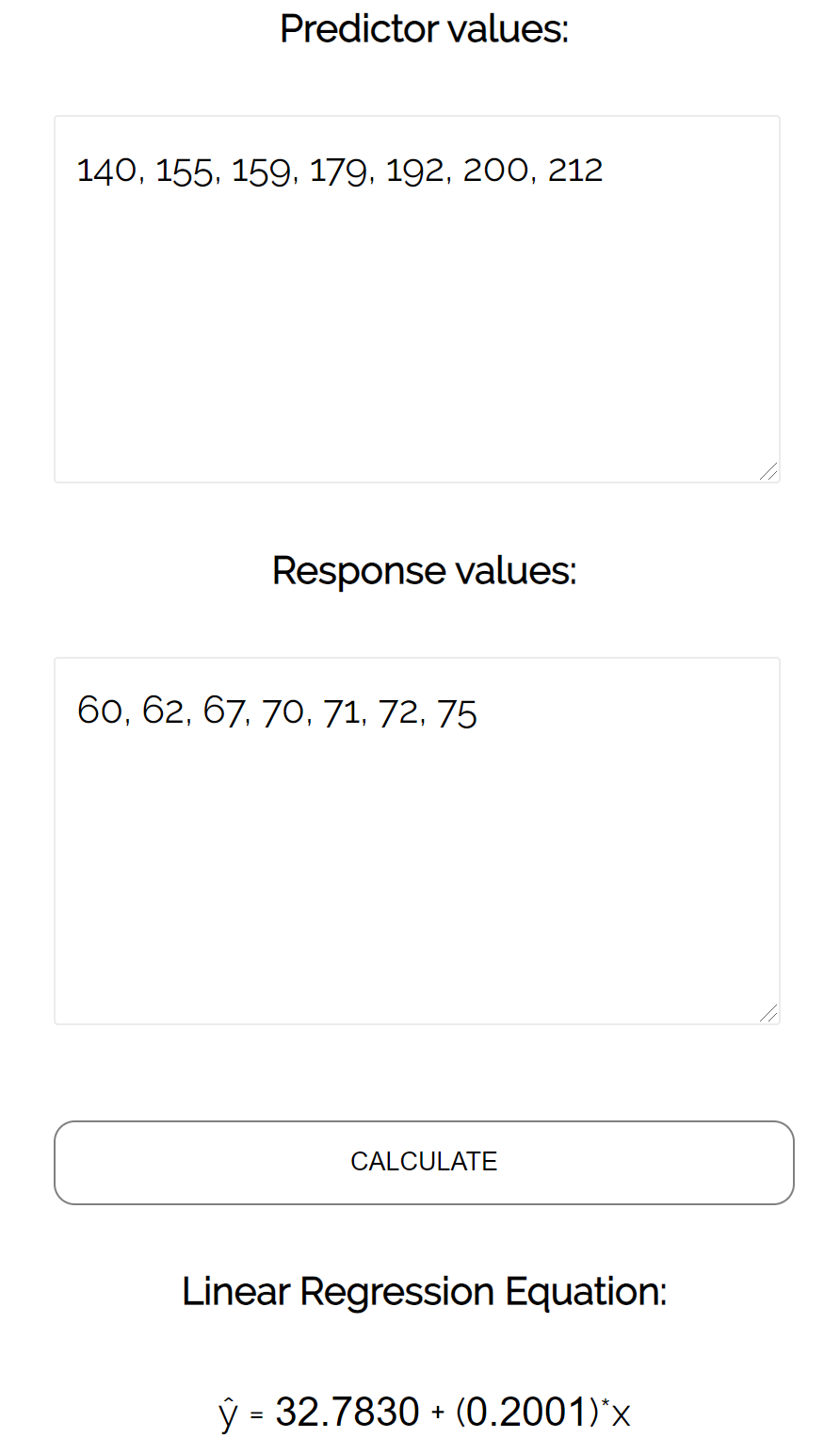
The calculator automatically finds the least squares regression line:
ŷ = 32.7830 + 0.2001x
If we zoom out on our scatterplot from earlier and added this line to the chart, here’s what it would look like:

Notice how our data points are scattered closely around this line. That’s because this least squares regression lines is the best fitting line for our data out of all the possible lines we could draw.
How to Interpret a Least Squares Regression Line
Here is how to interpret this least squares regression line: ŷ = 32.7830 + 0.2001x
b0 = 32.7830. This means when the predictor variable weight is zero pounds, the predicted height is 32.7830 inches. Sometimes the value for b0 can be useful to know, but in this specific example it doesn’t actually make sense to interpret b0 since a person can’t weight zero pounds.
b1 = 0.2001. This means that a one unit increase in x is associated with a 0.2001 unit increase in y. In this case, a one pound increase in weight is associated with a 0.2001 inch increase in height.
How to Use the Least Squares Regression Line
Using this least squares regression line, we can answer questions like:
For a person who weighs 170 pounds, how tall would we expect them to be?
To answer this, we can simply plug in 170 into our regression line for x and solve for y:
ŷ = 32.7830 + 0.2001(170) = 66.8 inches
For a person who weighs 150 pounds, how tall would we expect them to be?
To answer this, we can plug in 150 into our regression line for x and solve for y:
ŷ = 32.7830 + 0.2001(150) = 62.798 inches
Caution: When using a regression equation to answer questions like these, make sure you only use values for the predictor variable that are within the range of the predictor variable in the original dataset we used to generate the least squares regression line. For example, the weights in our dataset ranged from 140 lbs to 212 lbs, so it only makes sense to answer questions about predicted height when the weight is between 140 lbs and 212 lbs.
The Coefficient of Determination
One way to measure how well the least squares regression line “fits” the data is using the coefficient of determination, denoted as R2.
The coefficient of determination is the proportion of the variance in the response variable that can be explained by the predictor variable.
The coefficient of determination can range from 0 to 1. A value of 0 indicates that the response variable cannot be explained by the predictor variable at all. A value of 1 indicates that the response variable can be perfectly explained without error by the predictor variable.
An R2 between 0 and 1 indicates just how well the response variable can be explained by the predictor variable. For example, an R2 of 0.2 indicates that 20% of the variance in the response variable can be explained by the predictor variable; an R2 of 0.77 indicates that 77% of the variance in the response variable can be explained by the predictor variable.
Notice in our output from earlier we got an R2 of 0.9311, which indicates that 93.11% of the variability in height can be explained by the predictor variable of weight:
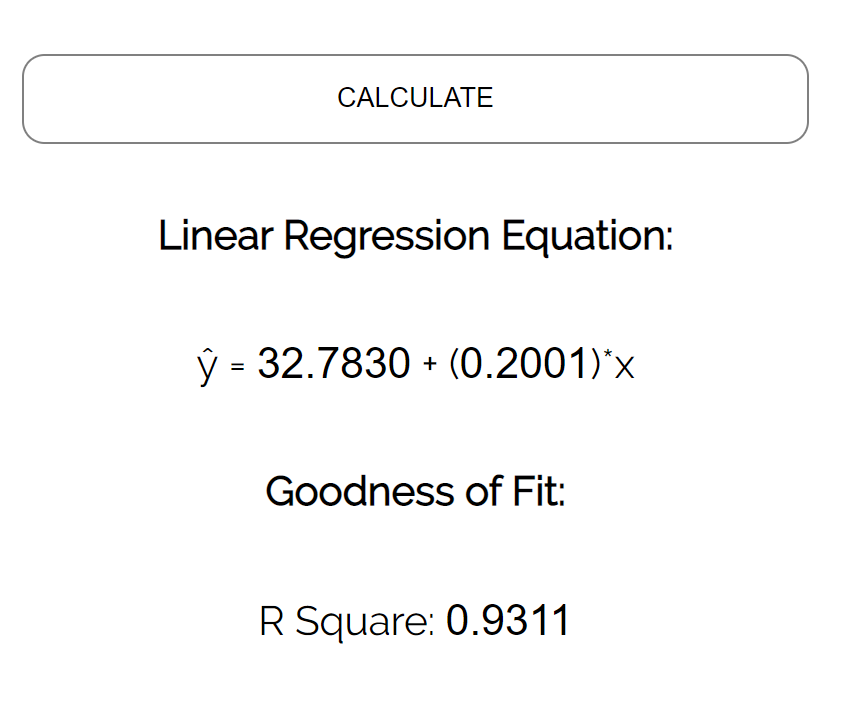
This tells us that weight is a very good predictor of height.
Assumptions of Linear Regression
For the results of a linear regression model to be valid and reliable, we need to check that the following four assumptions are met:
1. Linear relationship: There exists a linear relationship between the independent variable, x, and the dependent variable, y.
2. Independence: The residuals are independent. In particular, there is no correlation between consecutive residuals in time series data.
3. Homoscedasticity: The residuals have constant variance at every level of x.
4. Normality: The residuals of the model are normally distributed.
If one or more of these assumptions are violated, then the results of our linear regression may be unreliable or even misleading.
Refer to this post for an explanation for each assumption, how to determine if the assumption is met, and what to do if the assumption is violated.