Clustering is a technique in machine learning that attempts to find groups or clusters of observations within a dataset such that the observations within each cluster are quite similar to each other, while observations in different clusters are quite different from each other.
Clustering is a form of unsupervised learning because we’re simply attempting to find structure within a dataset rather than predicting the value of some response variable.
Clustering is often used in marketing when companies have access to information like:
- Household income
- Household size
- Head of household Occupation
- Distance from nearest urban area
When this information is available, clustering can be used to identify households that are similar and may be more likely to purchase certain products or respond better to a certain type of advertising.
One of the most common forms of clustering is known as k-means clustering. Unfortunately this method requires us to pre-specify the number of clusters K.
An alternative to this method is known as hierarchical clustering, which does not require us to pre-specify the number of clusters to be used and is also able to produce a tree-based representation of the observations known as a dendrogram.
What is Hierarchical Clustering?
Similar to k-means clustering, the goal of hierarchical clustering is to produce clusters of observations that are quite similar to each other while the observations in different clusters are quite different from each other.
In practice, we use the following steps to perform hierarchical clustering:
1. Calculate the pairwise dissimilarity between each observation in the dataset.
- First, we must choose some distance metric – like the Euclidean distance – and use this metric to compute the dissimilarity between each observation in the dataset.
- For a dataset with n observations, there will be a total of n(n-1)/2 pairwise dissimilarities.
2. Fuse observations into clusters.
- At each step in the algorithm, fuse together the two observations that are most similar into a single cluster.
- Repeat this procedure until all observations are members of one large cluster. The end result is a tree, which can be plotted as a dendrogram.
To determine how close together two clusters are, we can use a few different methods including:
- Complete linkage clustering: Find the max distance between points belonging to two different clusters.
- Single linkage clustering: Find the minimum distance between points belonging to two different clusters.
- Mean linkage clustering: Find all pairwise distances between points belonging to two different clusters and then calculate the average.
- Centroid linkage clustering: Find the centroid of each cluster and calculate the distance between the centroids of two different clusters.
- Ward’s minimum variance method: Minimize the total
Depending on the structure of the dataset, one of these methods may tend to produce better (i.e. more compact) clusters than the other methods.
Hierarchical Clustering in R
The following tutorial provides a step-by-step example of how to perform hierarchical clustering in R.
Step 1: Load the Necessary Packages
First, we’ll load two packages that contain several useful functions for hierarchical clustering in R.
library(factoextra)
library(cluster)
Step 2: Load and Prep the Data
For this example we’ll use the USArrests dataset built into R, which contains the number of arrests per 100,000 residents in each U.S. state in 1973 for Murder, Assault, and Rape along with the percentage of the population in each state living in urban areas, UrbanPop.
The following code shows how to do the following:
- Load the USArrests dataset
- Remove any rows with missing values
- Scale each variable in the dataset to have a mean of 0 and a standard deviation of 1
#load data
df #remove rows with missing values
df omit(df)

#scale each variable to have a mean of 0 and sd of 1
df #view first six rows of dataset
head(df)

               Murder   Assault   UrbanPop         Rape
Alabama    1.24256408 0.7828393 -0.5209066 -0.003416473
Alaska     0.50786248 1.1068225 -1.2117642  2.484202941
Arizona    0.07163341 1.4788032  0.9989801  1.042878388
Arkansas   0.23234938 0.2308680 -1.0735927 -0.184916602
California 0.27826823 1.2628144  1.7589234  2.067820292
Colorado   0.02571456 0.3988593  0.8608085  1.864967207
Step 3: Find the Linkage Method to Use
To perform hierarchical clustering in R we can use the agnes() function from the cluster package, which uses the following syntax:
agnes(data, method)
where:
- data: Name of the dataset.
- method: The method to use to calculate dissimilarity between clusters.
Since we don’t know beforehand which method will produce the best clusters, we can write a short function to perform hierarchical clustering using several different methods.
Note that this function calculates the agglomerative coefficient of each method, which is metric that measures the strength of the clusters. The closer this value is to 1, the stronger the clusters.
#define linkage methods
m #function to compute agglomerative coefficient
ac function(x) {
  agnes(df, method = x)$ac
}

#calculate agglomerative coefficient for each clustering linkage method
sapply(m, ac)

  average    single  complete      ward
0.7379371 0.6276128 0.8531583 0.9346210
We can see that Ward’s minimum variance method produces the highest agglomerative coefficient, thus we’ll use that as the method for our final hierarchical clustering:
#perform hierarchical clustering using Ward's minimum variance
clust ward")

#produce dendrogram
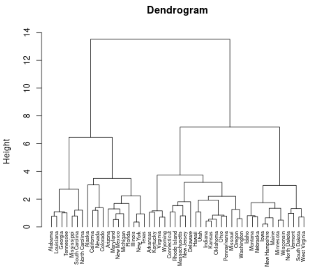
pltree(clust, cex = 0.6, hang = -1, main = "Dendrogram")

Each leaf at the bottom of the dendrogram represents an observation in the original dataset. As we move up the dendrogram from the bottom, observations that are similar to each other are fused together into a branch.
Step 4: Determine the Optimal Number of Clusters
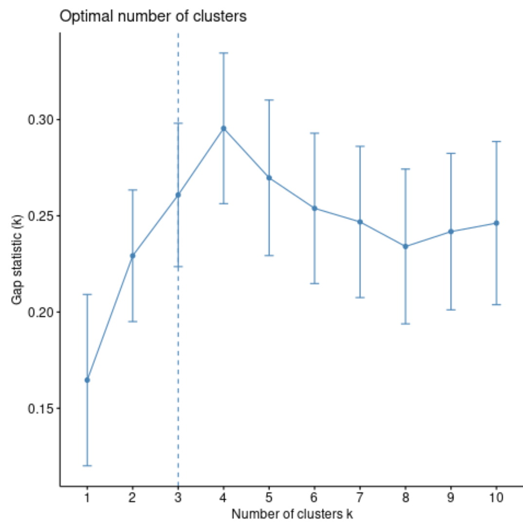
To determine how many clusters the observations should be grouped in, we can use a metric known as the gap statistic, which compares the total intra-cluster variation for different values of k with their expected values for a distribution with no clustering.
We can calculate the gap statistic for each number of clusters using the clusGap() function from the cluster package along with a plot of clusters vs. gap statistic using the fviz_gap_stat() function:
#calculate gap statistic for each number of clusters (up to 10 clusters)
gap_stat #produce plot of clusters vs. gap statistic
fviz_gap_stat(gap_stat)

From the plot we can see that the gap statistic is highest at k = 4 clusters. Thus, we’ll choose to group our observations into 4 distinct clusters.
Step 5: Apply Cluster Labels to Original Dataset
To actually add cluster labels to each observation in our dataset, we can use the cutree() method to cut the dendrogram into 4 clusters:
#compute distance matrix
d euclidean")

#perform hierarchical clustering using Ward's method
final_clust ward.D2" )

#cut the dendrogram into 4 clusters
groups #find number of observations in each cluster
table(groups)

 1  2  3  4
 7 12 19 12
We can then append the cluster labels of each state back to the original dataset:
#append cluster labels to original data
final_data
#display first six rows of final data
head(final_data)

               Murder Assault UrbanPop Rape cluster
Alabama          13.2     236       58 21.2       1
Alaska           10.0     263       48 44.5       2
Arizona           8.1     294       80 31.0       2
Arkansas          8.8     190       50 19.5       3
California        9.0     276       91 40.6       2
Colorado          7.9     204       78 38.7       2
Lastly, we can use the aggregate() function to find the mean of the variables in each cluster:
#find mean values for each cluster
aggregate(final_data, by=list(cluster=final_data$cluster), mean)

  cluster    Murder  Assault UrbanPop     Rape cluster
1       1 14.671429 251.2857 54.28571 21.68571       1
2       2 10.966667 264.0000 76.50000 33.60833       2
3       3  6.210526 142.0526 71.26316 19.18421       3
4       4  3.091667  76.0000 52.08333 11.83333       4
We interpret this output is as follows:
- The mean number of murders per 100,000 citizens among the states in cluster 1 is 14.67.
- The mean number of assaults per 100,000 citizens among the states in cluster 1 is 251.28.
- The mean percentage of residents living in an urban area among the states in cluster 1 is 54.28%.
- The mean number of rapes per 100,000 citizens among the states in cluster 1 is 21.68.
You can find the complete R code used in this example here.