Multiple linear regression is a method we can use to understand the relationship between several explanatory variables and a response variable.
Unfortunately, one problem that often occurs in regression is known as heteroscedasticity, in which there is a systematic change in the variance of residuals over a range of measured values.
This causes an increase in the variance of the regression coefficient estimates, but the regression model doesn’t pick up on this. This makes it much more likely for a regression model to declare that a term in the model is statistically significant, when in fact it is not.
One way to account for this problem is to use robust standard errors, which are more “robust” to the problem of heteroscedasticity and tend to provide a more accurate measure of the true standard error of a regression coefficient.
This tutorial explains how to use robust standard errors in regression analysis in Stata.
Example: Robust Standard Errors in Stata
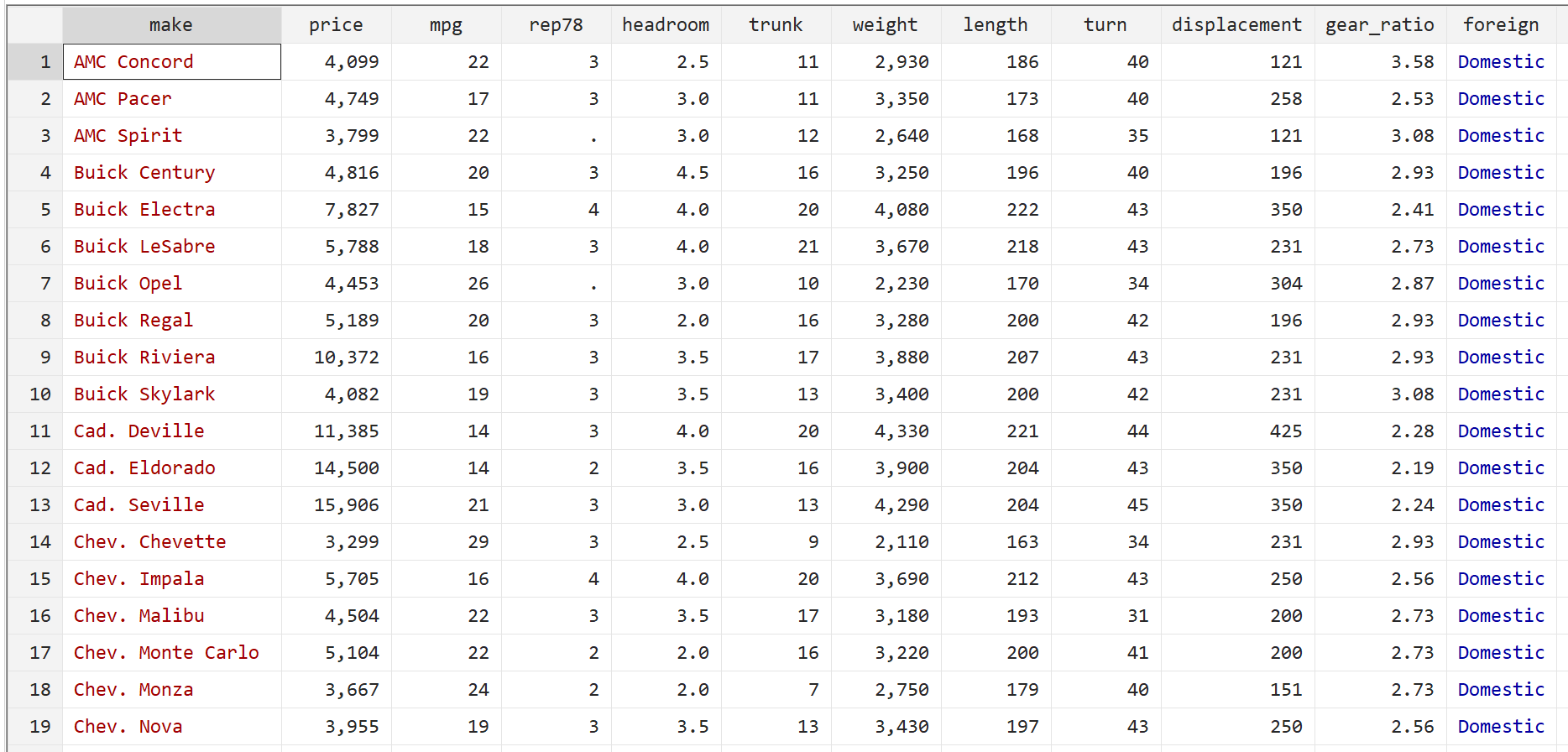
We will use the built-in Stata dataset auto to illustrate how to use robust standard errors in regression.
Step 1: Load and view the data.
First, use the following command to load the data:
sysuse auto
Then, view the raw data by using the following command:
br
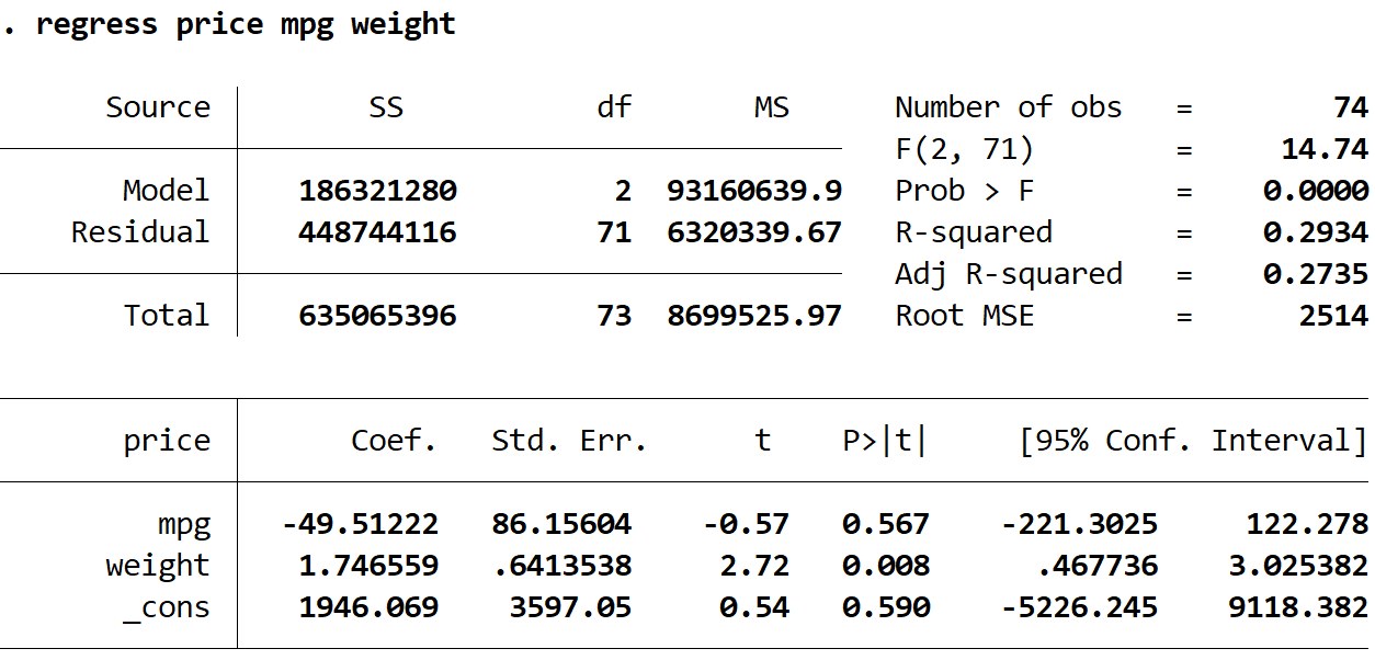
Step 2: Perform multiple linear regression without robust standard errors.
Next, we will type in the following command to perform a multiple linear regression using price as the response variable and mpg and weight as the explanatory variables:
regress price mpg weight
Step 3: Perform multiple linear regression using robust standard errors.
Now we will perform the exact same multiple linear regression, but this time we’ll use the vce(robust) command so Stata knows to use robust standard errors:
regress price mpg weight, vce(robust)
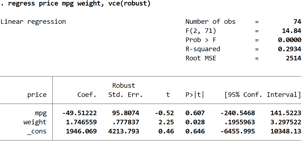
There are a few interesting things to note here:
1. The coefficient estimates remained the same. When we use robust standard errors, the coefficient estimates don’t change at all. Notice that the coefficient estimates for mpg, weight, and the constant are as follows for both regressions:
- mpg: -49.51222
- weight: 1.746559
- _cons: 1946.069
2. The standard errors changed. Notice that when we used robust standard errors, the standard errors for each of the coefficient estimates increased.
Note: In most cases, robust standard errors will be larger than the normal standard errors, but in rare cases it is possible for the robust standard errors to actually be smaller.
3. The test statistic of each coefficient changed. Notice that the absolute value of each test statistic, t, decreased. This is because the test statistic is calculated as the estimated coefficient divided by the standard error. Thus, the larger the standard error, the smaller the absolute value of the test statistic.
4. The p-values changed. Notice that the p-values for each variable also increased. This is because smaller test statistics are associated with larger p-values.
Although the p-values changed for our coefficients, the variable mpg is still not statistically significant at α = 0.05 and the variable weight is still statistically significant at α = 0.05.