In ordinary multiple linear regression, we use a set of p predictor variables and a response variable to fit a model of the form:
Y = β0 + β1X1 + β2X2 + … + βpXp + ε
where:
- Y: The response variable
- Xj: The jth predictor variable
- βj: The average effect on Y of a one unit increase in Xj, holding all other predictors fixed
- ε: The error term
The values for β0, β1, B2, … , βp are chosen using the least square method, which minimizes the sum of squared residuals (RSS):
RSS = Σ(yi – ŷi)2
where:
- Σ: A greek symbol that means sum
- yi: The actual response value for the ith observation
- ŷi: The predicted response value based on the multiple linear regression model
However, when the predictor variables are highly correlated then multicollinearity can become a problem. This can cause the coefficient estimates of the model to be unreliable and have high variance.
One way to get around this issue without completely removing some predictor variables from the model is to use a method known as ridge regression, which instead seeks to minimize the following:
RSS + λΣβj2
where j ranges from 1 to p and λ ≥ 0.
This second term in the equation is known as a shrinkage penalty.
When λ = 0, this penalty term has no effect and ridge regression produces the same coefficient estimates as least squares. However, as λ approaches infinity, the shrinkage penalty becomes more influential and the ridge regression coefficient estimates approach zero.
In general, the predictor variables that are least influential in the model will shrink towards zero the fastest.
Why Use Ridge Regression?
The advantage of ridge regression compared to least squares regression lies in the bias-variance tradeoff.
Recall that mean squared error (MSE) is a metric we can use to measure the accuracy of a given model and it is calculated as:
MSE = Var(f̂(x0)) + [Bias(f̂(x0))]2 + Var(ε)
MSE = Variance + Bias2 + Irreducible error
The basic idea of ridge regression is to introduce a little bias so that the variance can be substantially reduced, which leads to a lower overall MSE.
To illustrate this, consider the following chart:
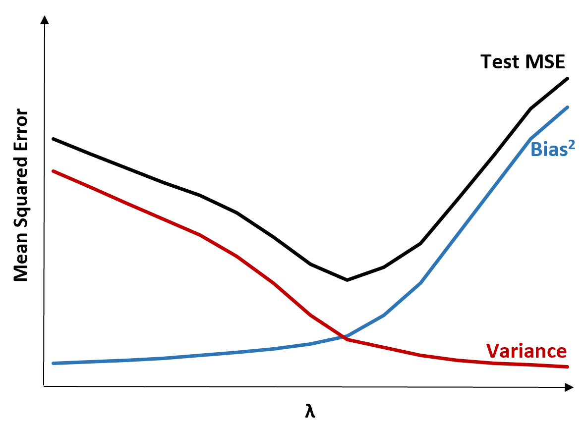
Notice that as λ increases, variance drops substantially with very little increase in bias. Beyond a certain point, though, variance decreases less rapidly and the shrinkage in the coefficients causes them to be significantly underestimated which results in a large increase in bias.
We can see from the chart that the test MSE is lowest when we choose a value for λ that produces an optimal tradeoff between bias and variance.
When λ = 0, the penalty term in ridge regression has no effect and thus it produces the same coefficient estimates as least squares. However, by increasing λ to a certain point we can reduce the overall test MSE.
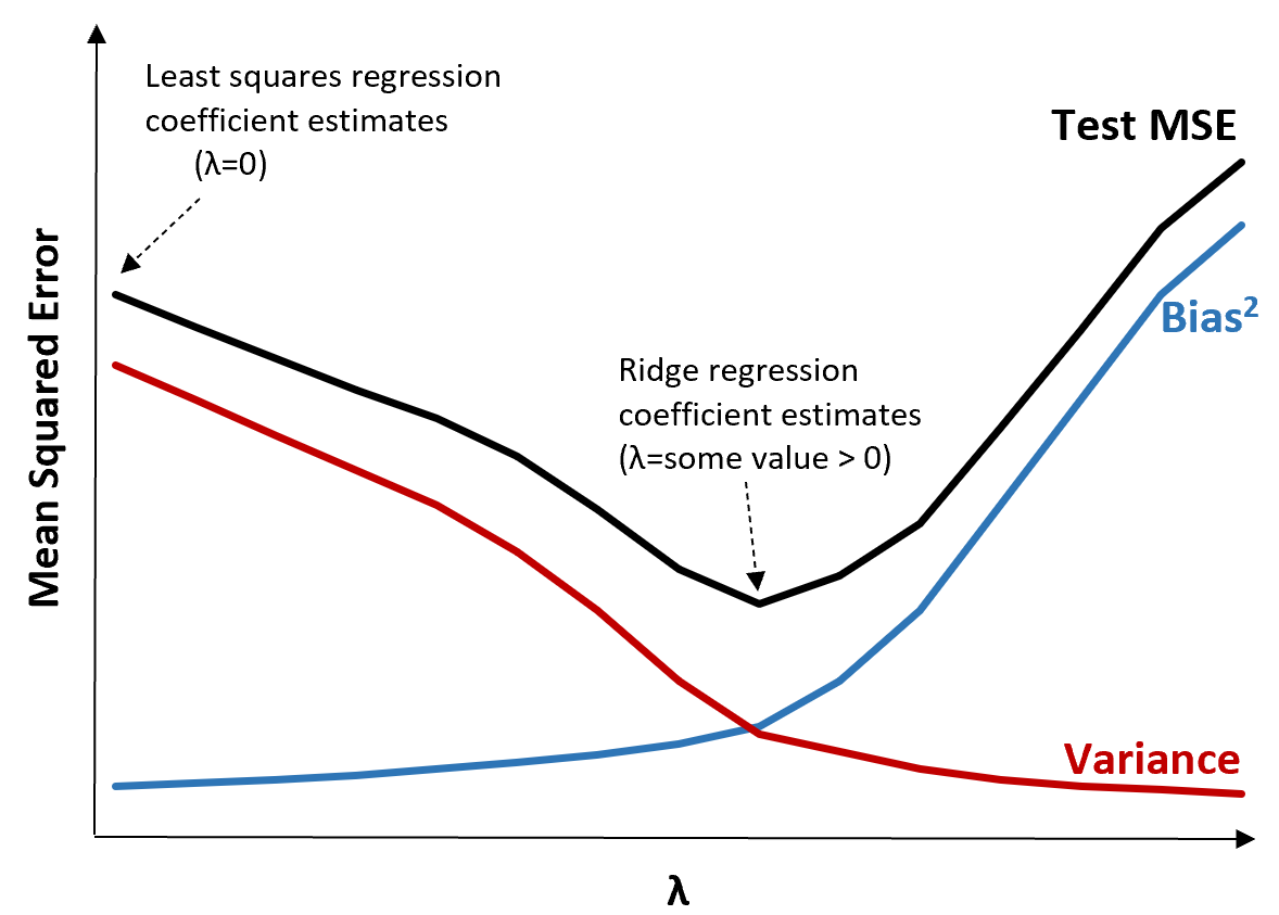
This means the model fit by ridge regression will produce smaller test errors than the model fit by least squares regression.
Steps to Perform Ridge Regression in Practice
The following steps can be used to perform ridge regression:
Step 1: Calculate the correlation matrix and VIF values for the predictor variables.
First, we should produce a correlation matrix and calculate the VIF (variance inflation factor) values for each predictor variable.
If we detect high correlation between predictor variables and high VIF values (some texts define a “high” VIF value as 5 while others use 10) then ridge regression is likely appropriate to use.
However, if there is no multicollinearity present in the data then there may be no need to perform ridge regression in the first place. Instead, we can perform ordinary least squares regression.
Step 2: Standardize each predictor variable.
Before performing ridge regression, we should scale the data such that each predictor variable has a mean of 0 and a standard deviation of 1. This ensures that no single predictor variable is overly influential when performing ridge regression.
Step 3: Fit the ridge regression model and choose a value for λ.
There is no exact formula we can use to determine which value to use for λ. In practice, there are two common ways that we choose λ:
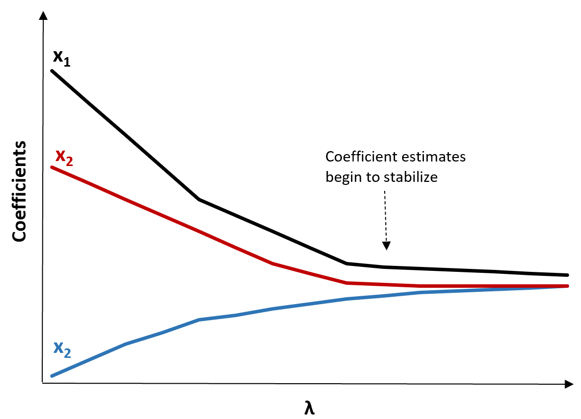
(1) Create a Ridge trace plot. This is a plot that visualizes the values of the coefficient estimates as λ increases towards infinity. Typically we choose λ as the value where most of the coefficient estimates begin to stabilize.
(2) Calculate the test MSE for each value of λ.
Another way to choose λ is to simply calculate the test MSE of each model with different values of λ and choose λ to be the value that produces the lowest test MSE.
Pros & Cons of Ridge Regression
The biggest benefit of ridge regression is its ability to produce a lower test mean squared error (MSE) compared to least squares regression when multicollinearity is present.
However, the biggest drawback of ridge regression is its inability to perform variable selection since it includes all predictor variables in the final model. Since some predictors will get shrunken very close to zero, this can make it hard to interpret the results of the model.
In practice, ridge regression has the potential to produce a model that can make better predictions compared to a least squares model but it is often harder to interpret the results of the model.
Depending on whether model interpretation or prediction accuracy is more important to you, you may choose to use ordinary least squares or ridge regression in different scenarios.
Ridge Regression in R & Python
The following tutorials explain how to perform ridge regression in R and Python, the two most common languages used for fitting ridge regression models:
Ridge Regression in R (Step-by-Step)
Ridge Regression in Python (Step-by-Step)