Imagine there exists a population of 10,000 dolphins and the mean weight of a dolphin in this population is 300 pounds.
If we take a simple random sample of 50 dolphins from this population, we might find that the mean weight of dolphins in this sample is 305 pounds.
Then if we take another simple random sample of 50 dolphins, we might find that the mean weight of dolphins in that sample is 295 pounds.
Each time we take a simple random sample of 50 dolphins, it’s likely that the mean weight of the dolphins in the sample will be close to the population mean of 300 pounds, but not exactly 300 pounds.
Imagine that we take 200 simple random samples of 50 dolphins from this population and make a histogram of the mean weight in each sample:
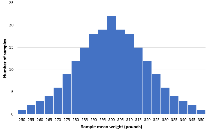
In most of the samples, the mean weight will be close to 300 pounds. In rare scenarios, we may happen to pick a sample full of small dolphins where the mean weight is only 250 pounds. Or we may happen to pick a sample full of large dolphins where the mean weight is 350 pounds. In general, the distribution of the sample means will be approximately normal with the center of the distribution located at the true center of the population.
This distribution of sample means is known as the sampling distribution of the mean and has the following properties:
μx = μ
where μx is the sample mean and μ is the population mean.
σx = σ/ √n
where σx is the sample standard deviation, σ is the population standard deviation, and n is the sample size.
For example, in this population of dolphins we know that the mean weight is μ = 300. So the mean of the sampling distribution is μx = 300.
Suppose we also know that the standard deviation of the population is 18 pounds. So the sample standard deviation is σx = 18/ √50 = 2.546.
Sampling Distribution of the Proportion
Consider the same population of 10,000 dolphins. Suppose 10% of the dolphins are black and the rest are gray. Suppose we take a simple random sample of 50 dolphins and find that 14% of the dolphins in that sample are black. Then we take another simple random sample of 50 dolphins and find that 8% of the dolphins in that sample are black.
Imagine that we take 200 simple random samples of 50 dolphins from this population and make a histogram of the proportion of dolphins that are black in each sample:
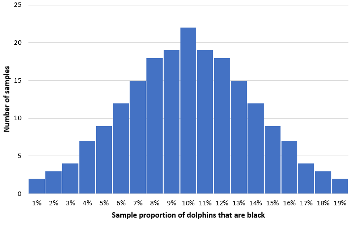
In most of the samples, the proportion of dolphins that are black will be close to the true population of 10%. The distribution of the sample proportion of dolphins that are black will be approximately normal with the center of the distribution located at the true center of the population.
This distribution of sample proportions is known as the sampling distribution of the proportion and has the following properties:
μp = P
where p is the sample proportion and P is the population proportion.
σp = √(P)(1-P) / n
where P is the population proportion and n is the sample size.
For example, in this population of dolphins we know that the true proportion of dolphins that are black is 10% = 0.1. So the mean of the sampling distribution of the proportion is μp = 0.1.
Suppose we also know that the standard deviation of the population is 18 pounds. So the sample standard deviation is σp = √(P)(1-P) / n = √(.1)(1-.1) / 50 = .042.
Establishing Normality
To use the formulas above, the sampling distribution needs to be normal.
According to the central limit theorem, the sampling distribution of a sample mean is approximately normal if the sample size is large enough, even if the population distribution is not normal. In most cases, we consider a sample size of 30 or larger to be sufficiently large.
The sampling distribution of a sample proportion is approximately normal if the expected number of successes and failures are both at least 10.
Examples
We can use sampling distributions to calculate probabilities.
Example 1: A certain machine creates cookies. The distribution of the weight of these cookies is skewed to the right with a mean of 10 ounces and a standard deviation of 2 ounces. If we take a simple random sample of 100 cookies produced by this machine, what is the probability that the mean weight of the cookies in this sample is less than 9.8 ounces?
Step 1: Establish normality.
We need to make sure that the sampling distribution of the sample mean is normal. Since our sample size is greater than or equal to 30, according to the central limit theorem we can assume that the sampling distribution of the sample mean is normal.
Step 2: Find the mean and standard deviation of the sampling distribution.
μx = μ
σx = σ/ √n
μx = 10 ounces
σx = 2/ √100 = 2/10 = 0.2 ounces
Step 3: Use the Z Score Area Calculator to find the probability that the mean weight of the cookies in this sample is less than 9.8 ounces.
Enter the following numbers into the Z Score Area Calculator. You can leave “Raw Score 2” blank since we’re only finding one number in this example.
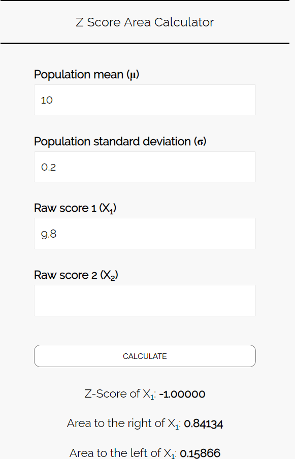
Since we want to know the probability that the mean weight of the cookies in this sample is less than 9.8 ounces, we are interested in the area to the left of 9.8. The calculator tells us that this probability is 0.15866.
Example 2: According to a school-wide study, 87% of students in a particular school prefer pizza over ice cream. Suppose we take a simple random sample of 200 students. What is the probability that the proportion of students who prefer pizza is less than 85%?
Step 1: Establish normality.
Recall that the sampling distribution of a sample proportion is approximately normal if the expected number of “successes” and “failures” are both at least 10.
In this case the expected number of students who will prefer pizza is 87% * 200 students = 174 students. The expected number of students who will not prefer pizza is 13% * 200 students = 26 students. Since both of these numbers are at least 10, we can assume that the sampling distribution of the sample proportion of students who will prefer pizza is approximately normal.
Step 2: Find the mean and standard deviation of the sampling distribution.
μp = P
σp = √(P)(1-P) / n
μp = 0.87
σp = √(.87)(1-.87) / 200 = .024
Step 3: Use the Z Score Area Calculator to find the probability that the proportion of students who prefer pizza is less than 85%.
Enter the following numbers into the Z Score Area Calculator. You can leave “Raw Score 2” blank since we’re only finding one number in this example.
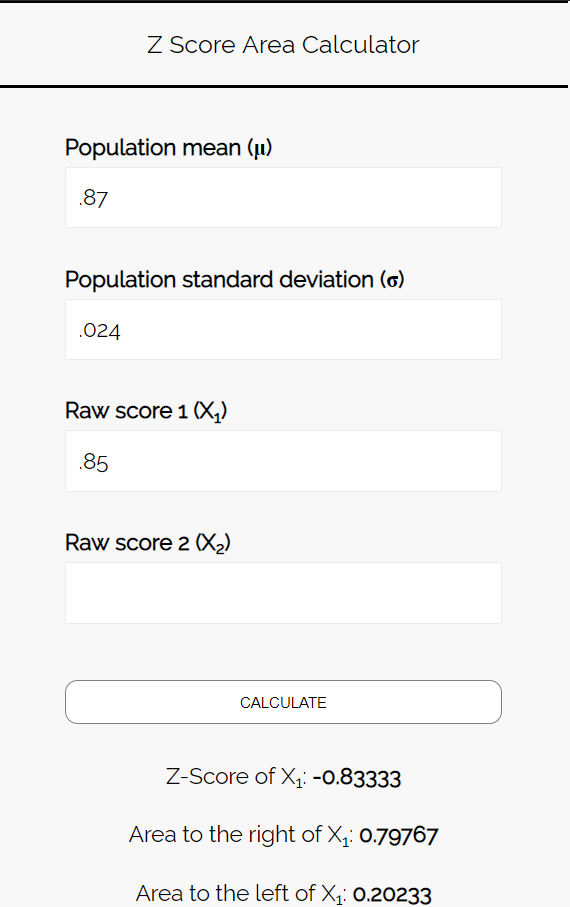
Since we want to know the probability that the proportion of students who prefer pizza is less than 85%, we are interested in the area to the left of 0.85. The calculator tells us that this probability is 0.20233.