When we want to understand the relationship between one or more predictor variables and a continuous response variable, we often use linear regression.
However, when the response variable is categorical we can instead use logistic regression.
Logistic regression is a type of classification algorithm because it attempts to “classify” observations from a dataset into distinct categories.
Here are a few examples of when we might use logistic regression:
- We want to use credit score and bank balance to predict whether or not a given customer will default on a loan. (Response variable = “Default” or “No default”)
- We want to use average rebounds per game and average points per game to predict whether or not a given basketball player will get drafted into the NBA (Response variable = “Drafted” or “Not Drafted”)
- We want to use square footage and number of bathrooms to predict whether or not a house in a certain city will be listed at a selling price of $200k or more. (Response variable = “Yes” or “No”)
Notice that the response variable in each of these examples can only take on one of two values. Contrast this with linear regression in which the response variable takes on some continuous value.
The Logistic Regression Equation
Logistic regression uses a method known as maximum likelihood estimation (details will not be covered here) to find an equation of the following form:
log[p(X) / (1-p(X))] = β0 + β1X1 + β2X2 + … + βpXp
where:
- Xj: The jth predictor variable
- βj: The coefficient estimate for the jth predictor variable
The formula on the right side of the equation predicts the log odds of the response variable taking on a value of 1.
Thus, when we fit a logistic regression model we can use the following equation to calculate the probability that a given observation takes on a value of 1:
p(X) = eβ0 + β1X1 + β2X2 + … + βpXp / (1 + eβ0 + β1X1 + β2X2 + … + βpXp)
We then use some probability threshold to classify the observation as either 1 or 0.
For example, we might say that observations with a probability greater than or equal to 0.5 will be classified as “1” and all other observations will be classified as “0.”
How to Interpret Logistic Regression Output
Suppose we use a logistic regression model to predict whether or not a given basketball player will get drafted into the NBA based on their average rebounds per game and average points per game.
Here is the output for the logistic regression model:
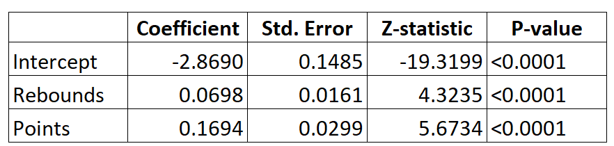
Using the coefficients, we can compute the probability that any given player will get drafted into the NBA based on their average rebounds and points per game using the following formula:
P(Drafted) = e-2.8690 + 0.0698*(rebs) + 0.1694*(points) / (1+e-2.8690 + 0.0698*(rebs) + 0.1694*(points))
For example, suppose a given player averages 8 rebounds per game and 15 points per game. According to the model, the probability that this player will get drafted into the NBA is 0.557.
P(Drafted) = e-2.8690 + 0.0698*(8) + 0.1694*(15) / (1+e-2.8690 + 0.0698*(8) + 0.1694*(15)) = 0.557
Since this probability is greater than 0.5, we would predict that this player will get drafted.
Contrast this with a player who only averages 3 rebounds and 7 points per game. The probability that this player will get drafted into the NBA is 0.186.
P(Drafted) = e-2.8690 + 0.0698*(3) + 0.1694*(7) / (1+e-2.8690 + 0.0698*(3) + 0.1694*(7)) = 0.186
Since this probability is less than 0.5, we would predict that this player will not get drafted.
Assumptions of Logistic Regression
Logistic regression uses the following assumptions:
1. The response variable is binary. It is assumed that the response variable can only take on two possible outcomes.
2. The observations are independent. It is assumed that the observations in the dataset are independent of each other. That is, the observations should not come from repeated measurements of the same individual or be related to each other in any way.
3. There is no severe multicollinearity among predictor variables. It is assumed that none of the predictor variables are highly correlated with each other.
4. There are no extreme outliers. It is assumed that there are no extreme outliers or influential observations in the dataset.
5. There is a linear relationship between the predictor variables and the logit of the response variable. This assumption can be tested using a Box-Tidwell test.
6. The sample size is sufficiently large. As a rule of thumb, you should have a minimum of 10 cases with the least frequent outcome for each explanatory variable. For example, if you have 3 explanatory variables and the expected probability of the least frequent outcome is 0.20, then you should have a sample size of at least (10*3) / 0.20 = 150.
Check out this post for a detailed explanation of how to check these assumptions.