You can use the following formula in Google Sheets to check if a cell contains text from a list:
=ArrayFormula(IF(LEN(A2:A13), REGEXMATCH(A2:A13,".*(?i)("&TEXTJOIN("|",
TRUE,$E$2:$E$4)&").*") ,""))
In this example, if cell A1 contains any of the text values in the range E2:E8 then it will return TRUE, otherwise it will return FALSE.
The following example shows how to use this formula in practice.
Example: Check if Cell Contains Text from List in Google Sheets
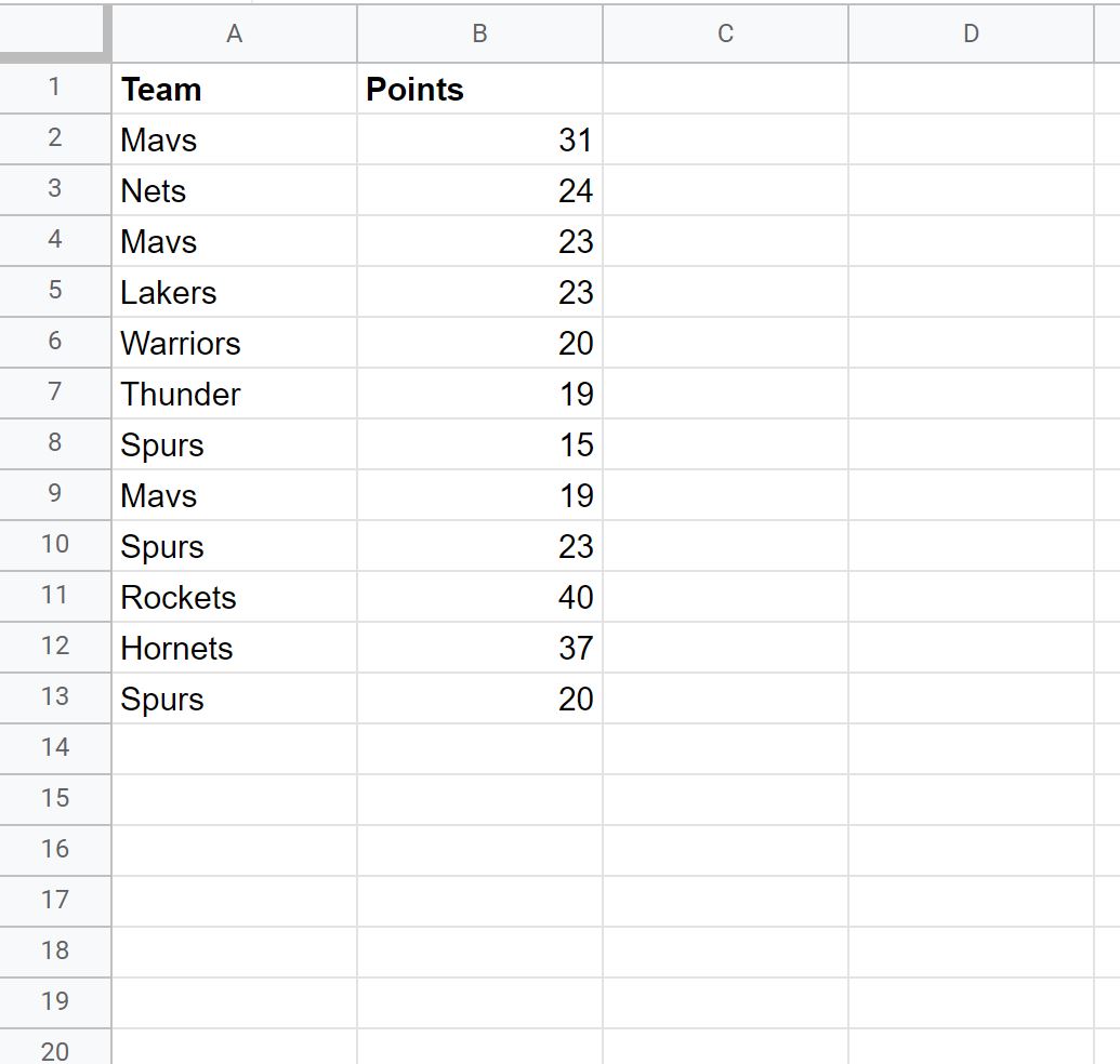
Suppose we have the following dataset in Google Sheets that shows the number of points scored by various basketball players:

There are three teams in the list from Texas: Mavs, Spurs, and Rockets.
Suppose we’d like to create a new column that tells us whether each team is from Texas or not.
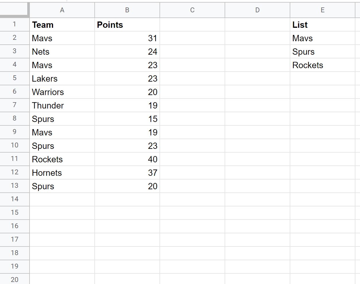
First, we’ll create a list of the Texas teams in column E:

Then we’ll use the following formula to check if the value in the Team column contains any of the text values in column E:
=ArrayFormula(IF(LEN(A2:A13), REGEXMATCH(A2:A13,".*(?i)("&TEXTJOIN("|",
TRUE,$E$2:$E$4)&").*") ,""))
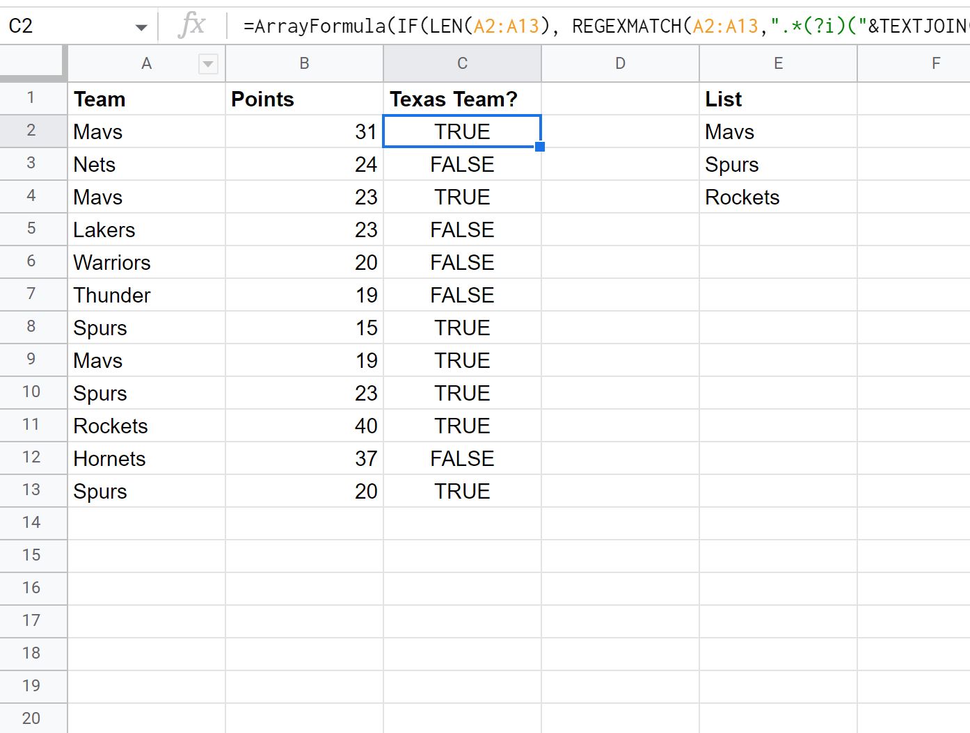
We can type this formula into cell C2 and then copy and paste it down to the remaining cells in column C:

Notice that any row that contains Mavs, Spurs, or Rockets receives a value of TRUE while all other rows receive a value of FALSE.
For example:
- The first row received a value of TRUE since “Mavs” is in the list.
- The second row received a value of FALSE since “Nets” is not in the list.
- The third row received a value of TRUE since “Mavs” is in the list.
- The fourth row received a value of FALSE since “Lakers” is not in the list.
And so on.
Additional Resources
The following tutorials explain how to perform other common tasks in Google Sheets:
How to Check if Cell is Empty in Google Sheets
How to Check if Value is in Range in Google Sheets
How to Use Conditional Formatting Based on Checkbox in Google Sheets