A one-way ANOVA is used to determine whether or not there is a statistically significant difference between the means of three or more independent groups.
This type of test is called a one-way ANOVA because we are analyzing how one predictor variable impacts a response variable.
If we were instead interested in how two predictor variables impact a response variable, we could conduct a two-way ANOVA.
This tutorial explains how to conduct a one-way ANOVA in SPSS.
Example: One-Way ANOVA in SPSS
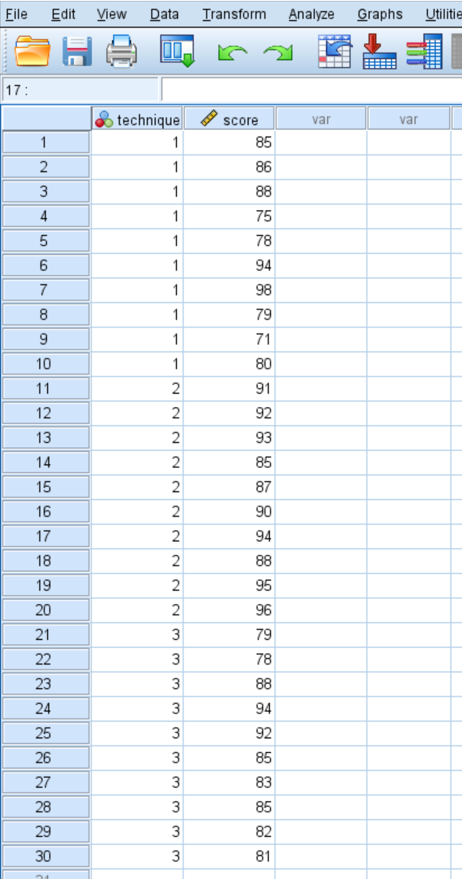
Suppose a researcher recruits 30 students to participate in a study. The students are randomly assigned to use one of three studying techniques for the next month to prepare for an exam. At the end of the month, all of the students take the same test.
The test scores for the students are shown below:
Use the following steps to perform a one-way ANOVA to determine if the average scores are the same across all three groups.
Step 1: Visualize the data.
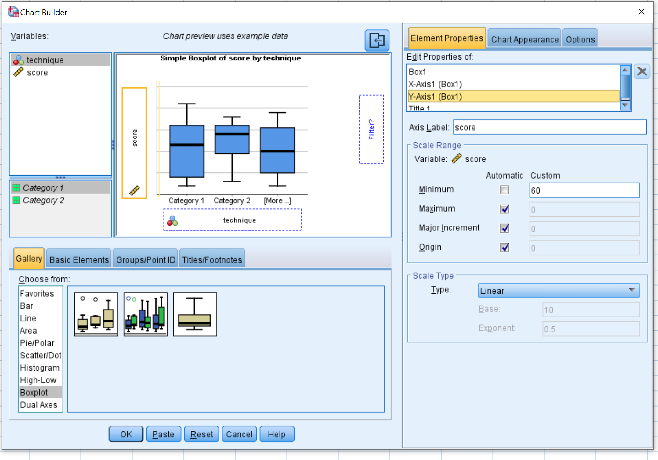
First, we’ll create boxplots to visualize the distribution of test scores for each of the three studying techniques. Click the Graphs tab, then click Chart Builder.

Select Boxplot in the Choose from: window. Then drag the first chart titled Simple boxplot into the main editing window. Drag the variable technique onto the x-axis and score onto the y-axis.
Then click Element Properties, then Y-axis1. Change the minimum value to 60. Then click OK.
The following boxplots will appear:
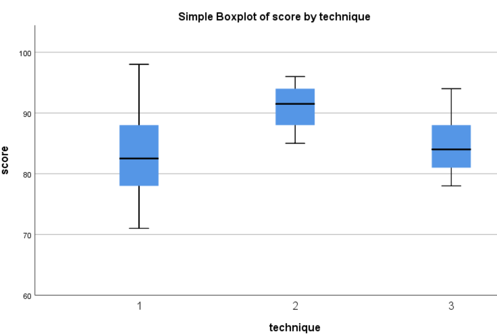
We can see that the distribution of test scores tend to be higher for students who used technique 2 compared to students who used techniques 1 and 3. To determine if these differences in scores are statistically significant, we’ll perform a one-way ANOVA.
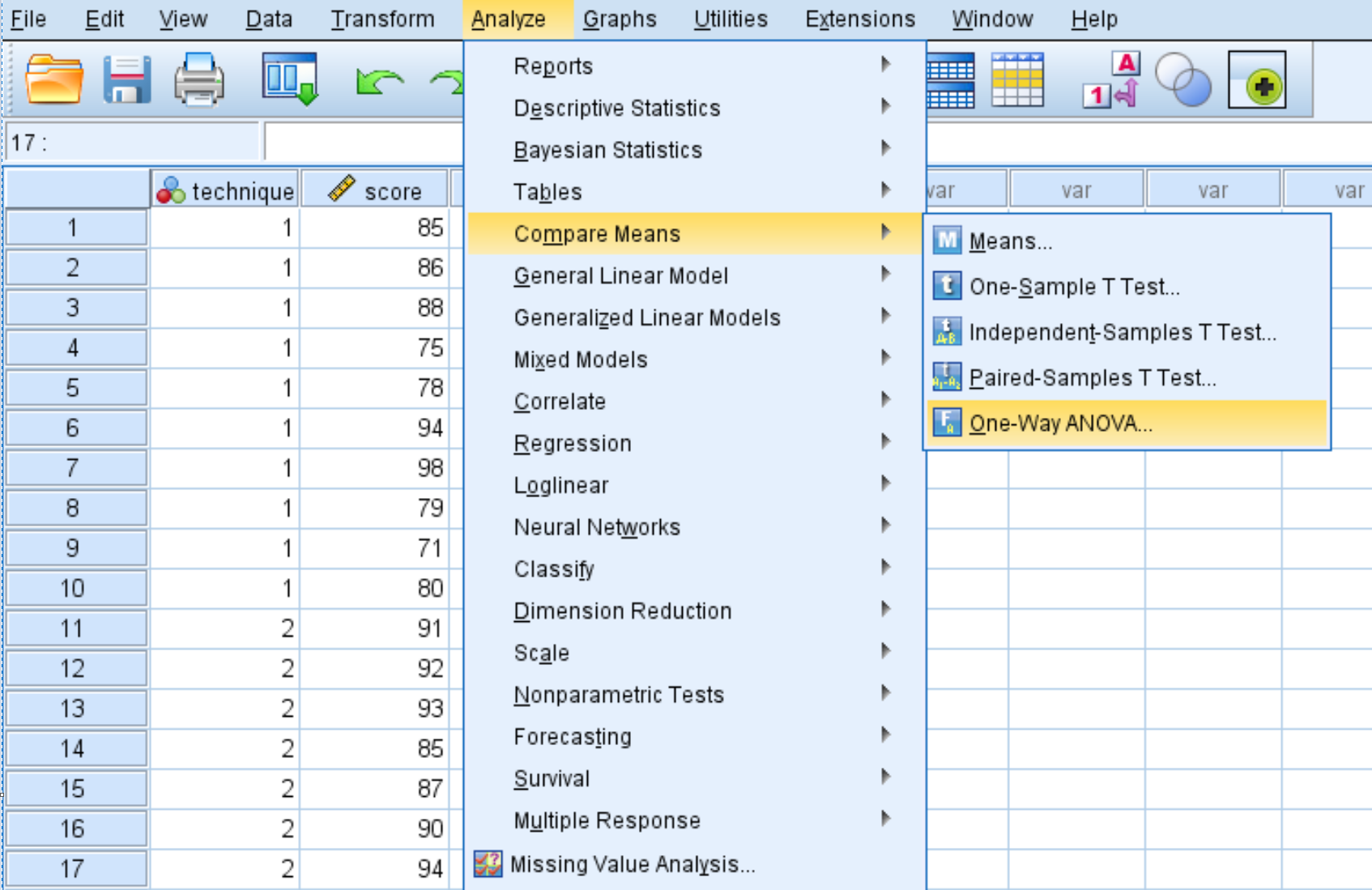
Step 2: Perform a one-way ANOVA.
Click the Analyze tab, then Compare Means, then One-Way ANOVA.
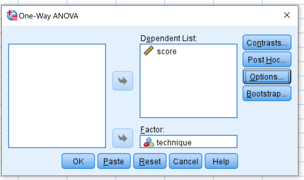
In the new window that pops up, place the variable score into the box labelled Dependent list and the variable technique into the box labelled Factor.
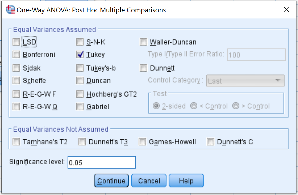
Then click Post Hoc and check the box next to Tukey. Then click Continue.
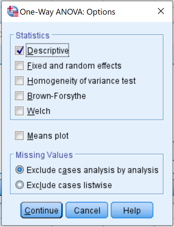
Then click Options and check the box next to Descriptive. Then click Continue.
Lastly, click OK.
Step 3: Interpret the output.
Once you click OK, the results of the one-way ANOVA will appear. Here is how to interpret the output:
Descriptives Table
This table displays descriptive statistics for each of the three groups in our dataset.
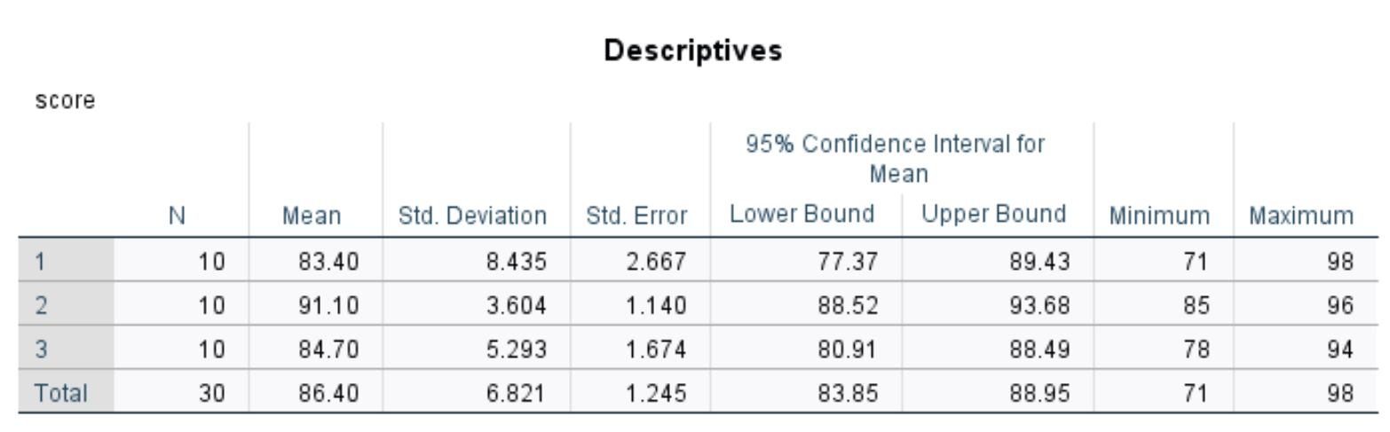
The most relevant numbers include:
- N: The number of students in each group.
- Mean: The mean test score for each group.
- Std. Deviation: The standard deviation of test scores for each group.
ANOVA Table
This table displays the results of the one-way ANOVA:
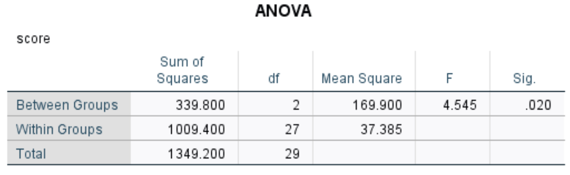
The most relevant numbers include:
- F: The overall F-statistic.
- Sig: The p-value that corresponds to the F-statistic (4.545) with df numerator (2) and df denominator (27). In this case, the p-value turns out to be .020.
Recall that a one-way ANOVA uses the following null and alternative hypotheses:
- H0 (null hypothesis): μ1 = μ2 = μ3 = … = μk (all the population means are equal)
- HA (alternative hypothesis): at least one population mean is different from the rest
Since the p-value from the ANOVA table is less than .05, we have sufficient evidence to reject the null hypothesis and conclude that at least one of the group means is different from the rest.
To find out exactly which group means differ from one another, we can refer to the last table in the ANOVA output.
Multiple Comparisons Table
This table displays the Tukey post-hoc multiple comparisons between each of the three groups. We are mostly interested in the Sig. column, which displays the p-values for the differences in means between each group:
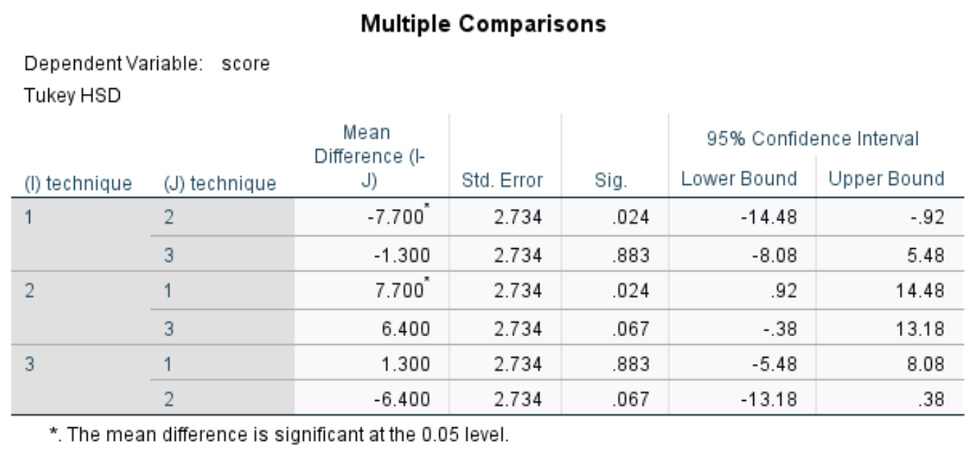
From the table we can see the p-values for the following comparisons:
- Technique 1 vs. 2: | p-value = 0.024
- Technique 1 vs. 3 | p-value = 0.883
- Technique 2 vs. 3 | p-value = 0.067
The only group comparison that has a p-value less than .05 is between technique 1 and technique 2.
This tells us that there is a statistically significant difference in average test scores between students who used technique 1 compared to students who used technique 2.
However, there is no statistically significant difference between technique 1 and 3, or between technique 2 and 3.
Step 4: Report the results.
Lastly, we can report the results of the one-way ANOVA. Here is an example of how to do so:
A one-way ANOVA was performed to determine if three different studying techniques lead to different test scores.
A total of 10 students used each of the three studying techniques for one month before all taking the same test.
A one-way ANOVA revealed that there was a statistically significant difference in test scores between at least two groups (F(2, 27) = 4.545, p = 0.020).
Tukey’s test for multiple comparisons found that mean test scores were significantly different between students who used technique 1 and technique 2 (p = .024, 95% C.I. = [-14.48, -.92]).
There was no statistically significant difference between scores for techniques 1 and 3 (p=.883) or between scores for techniques 2 and 3 (p = .067).