How to Perform a Chi-Square Goodness of Fit Test in Stata

---

A Chi-Square Goodness of Fit Test is used to determine whether or not a categorical variable follows a hypothesized distribution.

This tutorial explains how to perform a Chi-Square Goodness of Fit Test in Stata.

Example: Chi-Square Goodness of Fit Test in Stata

To illustrate how to perform this test, we will use a dataset called nlsw88, which contains information about labor statistics for women in the U.S. in 1988.

Use the following steps to perform a Chi-Square Goodness of Fit test to determine if the true distribution of race in this dataset is as follows: 70% White, 20% Black, 10% Other.

Step 1: Load and view the raw data.

First, we will load the data by typing in the following command:

sysuse nlsw88

We can view the raw data by typing in the following command:

br

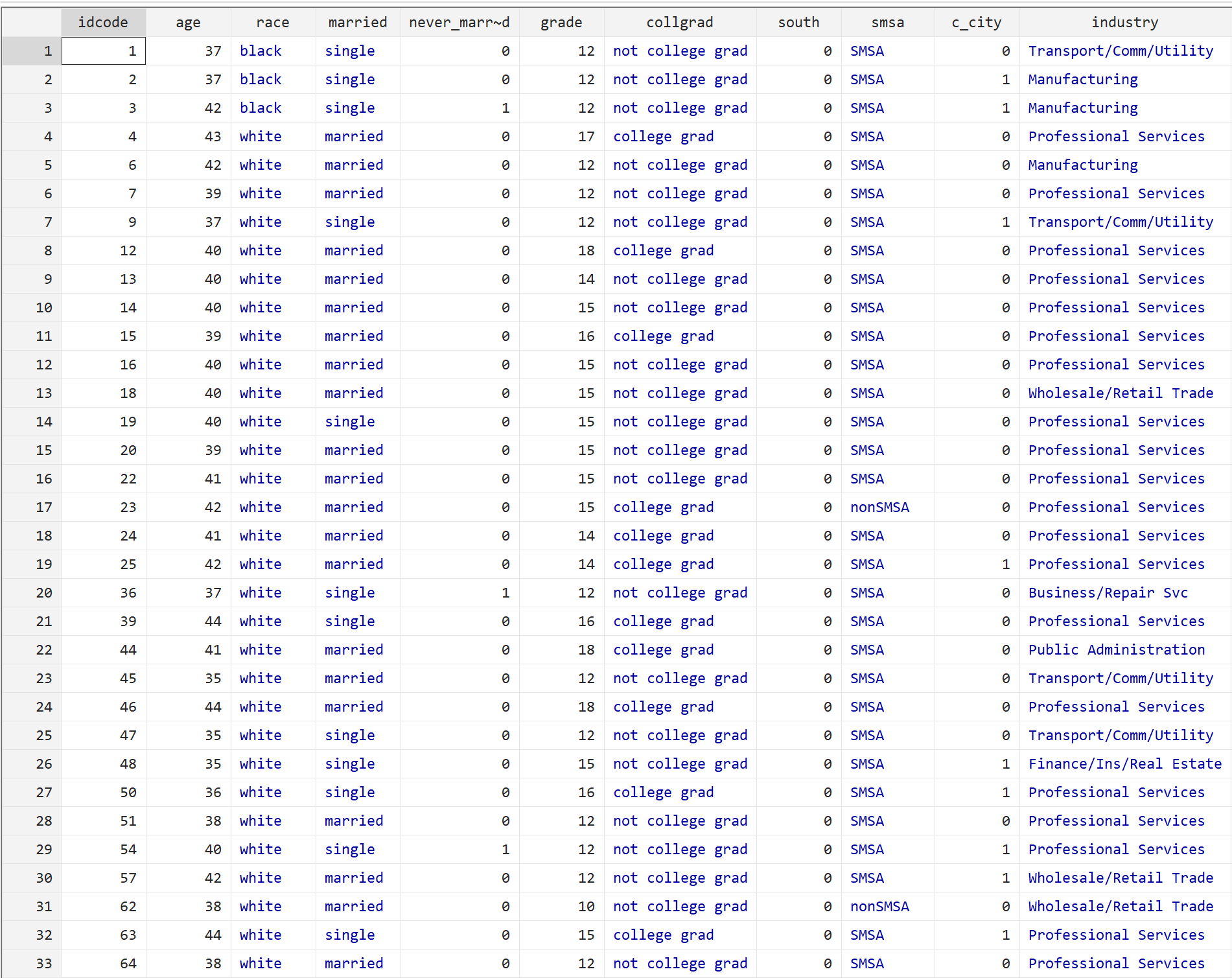
Each line displays information for an individual including their age, race, marital status, education level, and a variety of other factors.

Step 2: Load the goodness of fit package.

To perform a Goodness of Fit Test, we will need to install the csgof package. We can do so by typing in the following command:

findit csgof

A new window will pop up. Click the link that says csgof from https://stats.idre.ucla.edu/stat/stata/ado/analysis.

Another window will pop up. Click the link that says click here to install. 

The package should only take a few seconds to install.

Step 3: Perform the Goodness-of-Fit Test.

Once the package is installed, we can perform the Goodness of Fit Test on the data to determine if the true distribution of race is as follows: 70% White, 20% Black, 10% Other.

We will use the following syntax to perform the test:

csgof variable_of_interest, expperc(list_of_expected_percentages)

Here is the exact syntax we’ll use in our case:

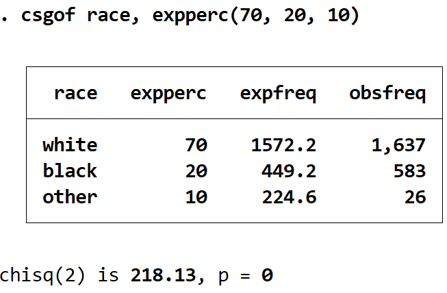
csgof race, expperc(70, 20, 10)

Here is how to interpret the output:

Summary box: This box shows us the expected percent, expected frequency, and observed frequency for each race. For example:

• The expected percent of white individuals was 70%. This is the percentage that we specified. 
• The expected frequency of white individuals was 1,572.2. This is calculated using the fact that there were 2,246 individuals in the dataset, so 70% of that number is 1,572.2.
• The observed frequency of white individuals was 1,637. This is the actual number of white individuals in the dataset.

Chisq(2): This is the Chi-Square test statistic for the Goodness of Fit Test. It turns out to be 218.13.

p: This is the p-value associated with the Chi-Square test statistic. It turns out to be 0. Since this is less than 0.05, we fail to reject the null hypothesis that the true distribution of race is 70% White, 20% Black, 10% Other. We have sufficient evidence to conclude that the true distribution of race is different from this hypothesized distribution.