A one-way ANOVA is used to determine whether or not different levels of an explanatory variable lead to statistically different results in some response variable.
For example, we might be interested in understanding whether or not three levels of education (Associate’s degree, Bachelor’s degree, Master’s degree) lead to statistically different annual incomes. In this case, we have one explanatory variable and one response variable.
- Explanatory variable: level of education
- Response variable: annual income
A MANOVA is an extension of the one-way ANOVA in which there is more than one response variable. For example, we might be interested in understanding whether or not level of education leads to different annual incomes and different amounts of student loan debt. In this case, we have one explanatory variable and two response variables:
- Explanatory variable: level of education
- Response variables: annual income, student loan debt
Because we have more than one response variable, it would be appropriate to use a MANOVA in this case.
Next, we’ll explain how to perform a MANOVA in Stata.
Example: MANOVA in Stata
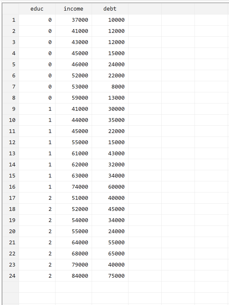
To illustrate how to perform a MANOVA in Stata, we’ll use the following dataset that contains the following three variables for 24 individuals:
- educ: level of education (0 = Associate, 1 = Bachelor, 2 = Master)
- income: annual income
- debt: total student loan debt
You can replicate this example by manually entering the data yourself by going to Data > Data Editor > Data Editor (Edit) along the top menu bar.
To perform the MANOVA using education as the explanatory variable and income and debt as the response variables, we can use the following command:
manova income debt = educ
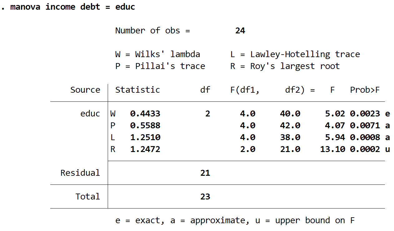
Stata produces four unique test statistics along with their corresponding p-values:
Wilks’ lambda: F-Statistic = 5.02, P-value = 0.0023.
Pillai’s trace: F-Statistic = 4.07, P-value = 0.0071.
Lawley-Hotelling trace: F-Statistic = 5.94, P-value = 0.0008.
Roy’s largest root: F-Statistic = 13.10, P-value = 0.0002.
For an in-depth explanation of how each test statistic is calculated, refer to this article from the Penn State Eberly College of Science.
The p-value for each test statistic is less than 0.05, so the null hypothesis will be rejected no matter which one you use. This means we have sufficient evidence to say that level of education leads to statistically significant differences in annual income and total student debt.
Note on p-values: The letter next to the p-value in the output table indicates how the F-statistic was calculated (e = exact calculation, a = approximate calculation, u = an upper bound).