Many statistical tests require one or more variables to be normally distributed in order for the results of the test to be reliable.
This tutorial explains several methods you can use to test for normality among variables in Stata.
For each of these methods, we will use the built-in Stata dataset called auto. You can load this dataset using the following command:
sysuse auto
Method 1: Histograms
One informal way to see if a variable is normally distributed is to create a histogram to view the distribution of the variable.
If the variable is normally distributed, the histogram should take on a “bell” shape with more values located near the center and fewer values located out on the tails.
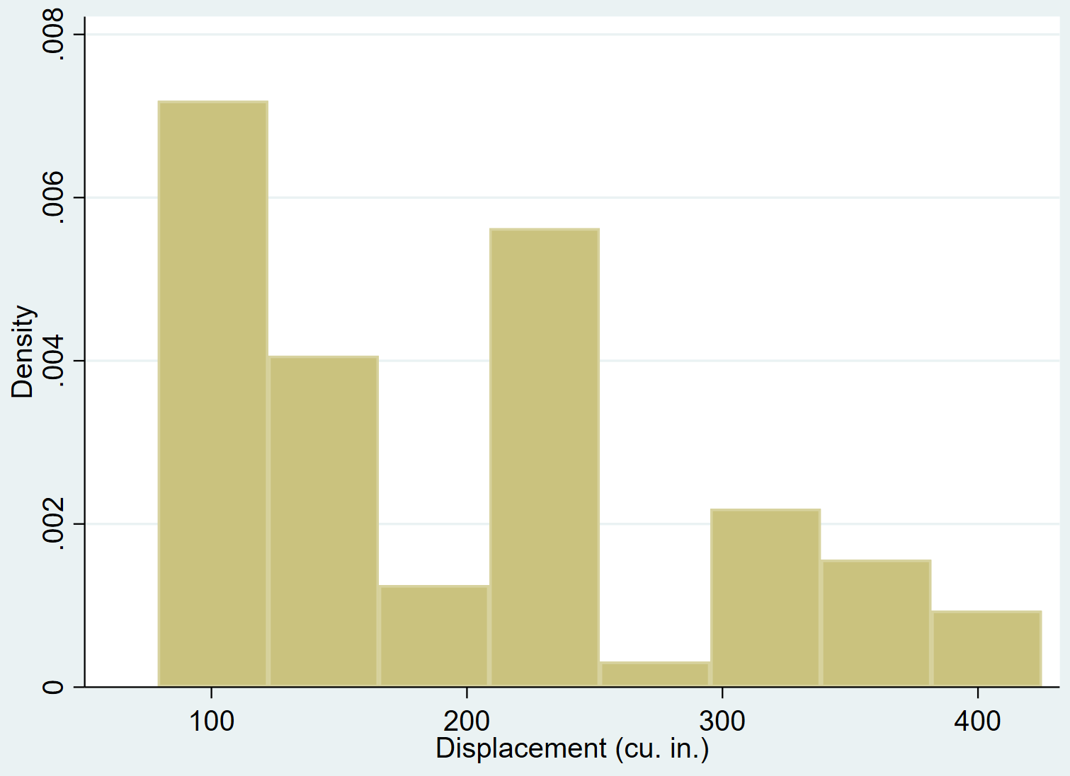
We can use the hist command to create a histogram for the variable displacement:
hist displacement
We can add a normal density curve to a histogram by using the normal command:
hist displacement, normal
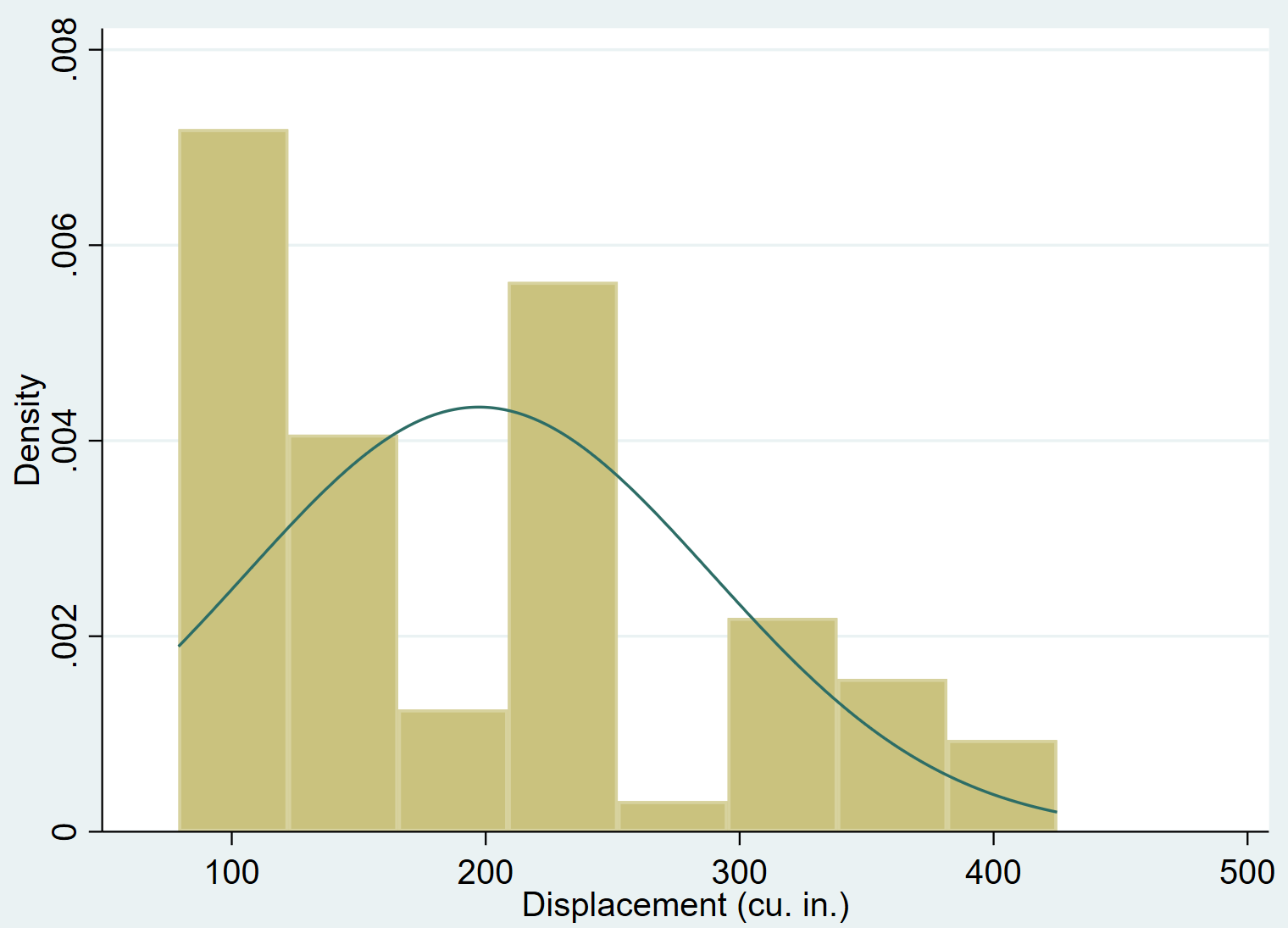
It’s pretty obvious that the variable displacement is skewed to the right (e.g. most values are concentrated on the left and a long “tail” of values extends to the right) and does not follow a normal distribution.
Related: Left Skewed vs. Right Skewed Distributions
Method 2: Shapiro-Wilk Test
A formal way to test for normality is to use the Shapiro-Wilk Test.
The null hypothesis for this test is that the variable is normally distributed. If the p-value of the test is less than some significance level (common choices include 0.01, 0.05, and 0.10), then we can reject the null hypothesis and conclude that there is sufficient evidence to say that the variable is not normally distributed.
*This test can be used when the total number of observations is between 4 and 2,000.
We can use the the swilk command to perform a Shapiro-Wilk Test on the variable displacement:
swilk displacement
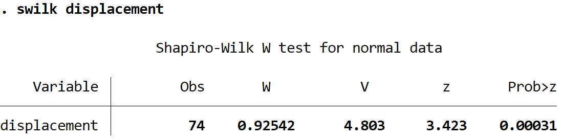
Here is how to interpret the output of the test:
Obs: 74. This is the number of observations used in the test.
W: 0.92542. This is the test statistic for the test.
Prob>z: 0.00031. This is the p-value associated with the test statistic.
Since the p-value is less than 0.05, we can reject the null hypothesis of the test. We have sufficient evidence to say that the variable displacement is not normally distributed.
We can also perform the Shapiro-Wilk Test on more than one variable at once by listing several variables after the swilk command:
swilk displacement mpg length
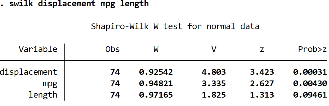
Using a 0.05 significance level, we would conclude that displacement and mpg are both non-normally distributed, but we don’t have sufficient evidence to say that length is non-normally distributed.
Method 3: Shapiro-Francia Test
Another formal way to test for normality is to use the Shapiro-Francia Test.
The null hypothesis for this test is that the variable is normally distributed. If the p-value of the test is less than some significance level, then we can reject the null hypothesis and conclude that there is sufficient evidence to say that the variable is not normally distributed.
*This test can be used when the total number of observations is between 10 and 5,000.
We can use the the sfrancia command to perform a Shapiro-Wilk Test on the variable displacement:
sfrancia displacement
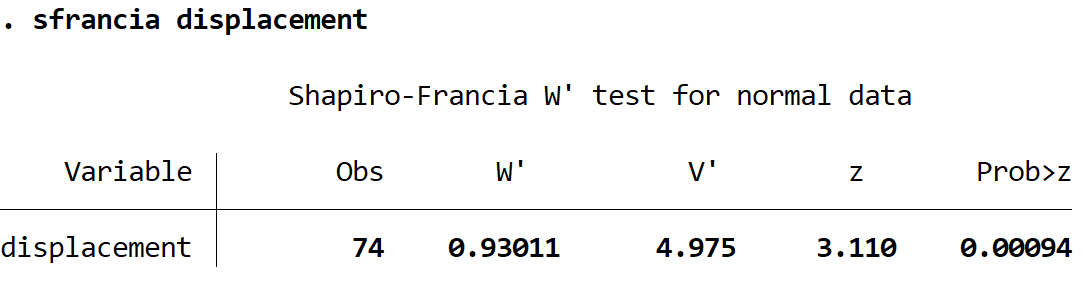
Here is how to interpret the output of the test:
Obs: 74. This is the number of observations used in the test.
W’: 0.93011. This is the test statistic for the test.
Prob>z: 0.00094. This is the p-value associated with the test statistic.
Since the p-value is less than 0.05, we can reject the null hypothesis of the test. We have sufficient evidence to say that the variable displacement is not normally distributed.
Similar to the Shapiro-Wilk Test, you can perform the Shapiro-Francia Test on more than one variable at once by listing several variables after the sfrancia command.
Method 4: Skewness and Kurtosis Test
Another way to test for normality is to use the Skewness and Kurtosis Test, which determines whether or not the skewness and kurtosis of a variable is consistent with the normal distribution.
The null hypothesis for this test is that the variable is normally distributed. If the p-value of the test is less than some significance level, then we can reject the null hypothesis and conclude that there is sufficient evidence to say that the variable is not normally distributed.
*This test requires a minimum of 8 observations to be used.
We can use the the sktest command to perform a Skewness and Kurtosis Test on the variable displacement:
sktest displacement
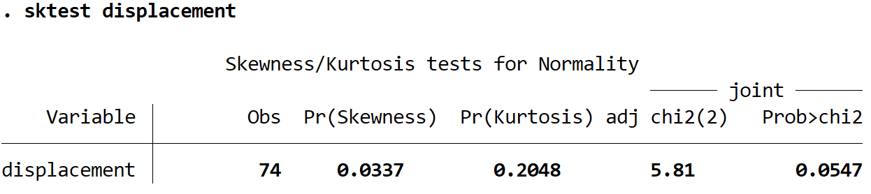
Here is how to interpret the output of the test:
Obs: 74. This is the number of observations used in the test.
adj chi(2): 5.81. This is the Chi-Square test statistic for the test.
Prob>chi2: 0.0547. This is the p-value associated with the test statistic.
Since the p-value is not less than 0.05, we fail to reject the null hypothesis of the test. We don’t have sufficient evidence to say that displacement is not normally distributed.
Similar to the other normality tests, you can perform the Skewness and Kurtosis Test on more than one variable at once by listing several variables after the sktest command.