You can use the IMPORTRANGE function in Google Sheets to import data from another spreadsheet.
To apply a filter to the IMPORTRANGE function, you can use the following syntax:
=FILTER(IMPORTRANGE("URL", "sheet1!A1:C12"),
        INDEX(IMPORTRANGE("URL", "sheet1!A1:C12"),0,2)="Spurs")
This particular example will import the cells in the range A1:C12 from the sheet called sheet1 from some workbook and filter the range to only show the rows where the value in column 2 is equal to “Spurs.”
The following example shows how to use this syntax in practice.
Example: How to Filter IMPORTRANGE Data
Suppose we would like to import data from a Google spreadsheet with a sheet named stats located at the following URL:
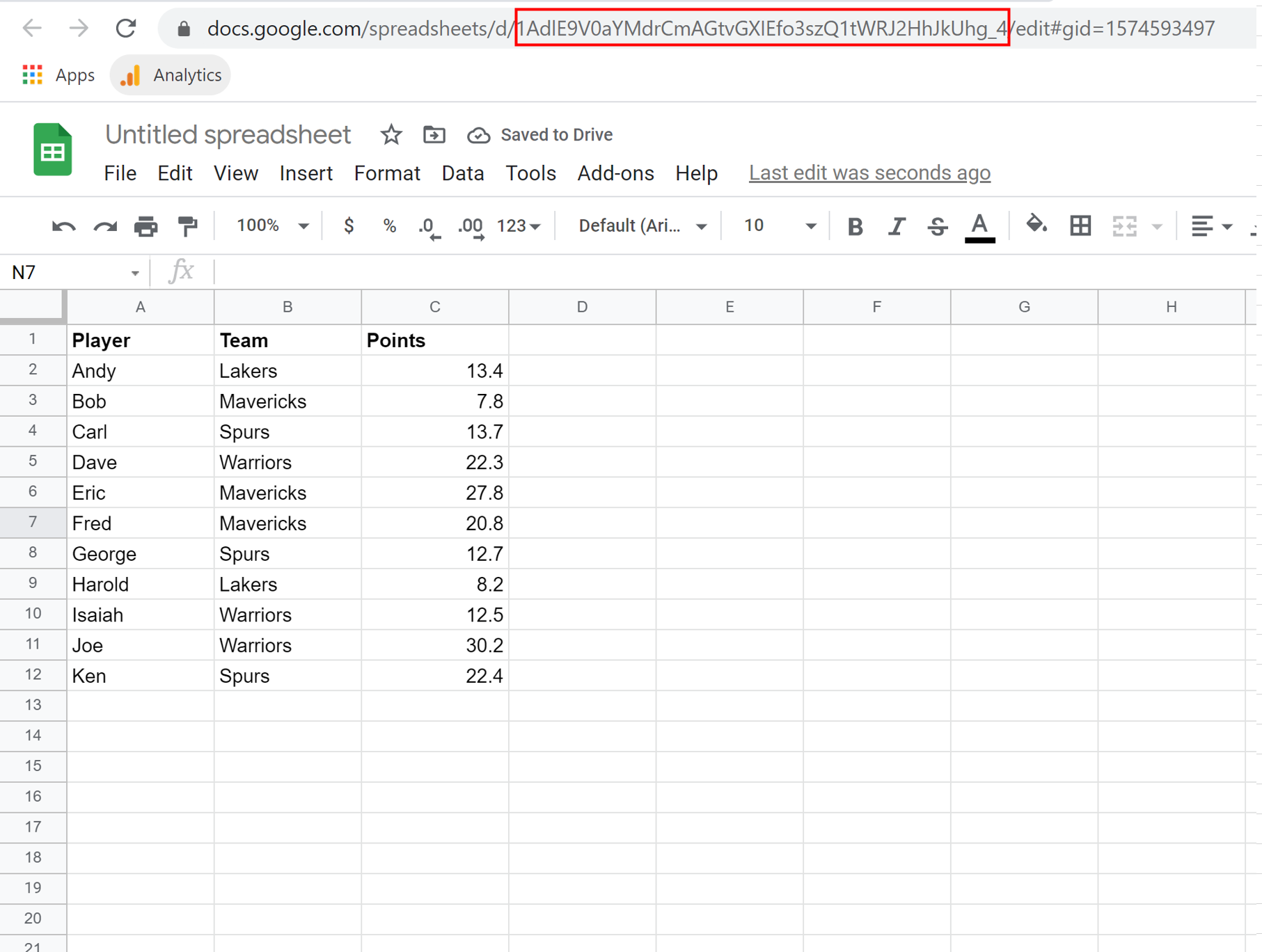
Also suppose that we would only like to import the rows where the value in the second column (the “Team” column) has a value of “Spurs.”
We can type the following formula into cell A1 of our current spreadsheet to import this particular data:
=FILTER(IMPORTRANGE("1AdlE9V0aYMdrCmAGtvGXIEfo3szQ1tWRJ2HhJkUhg_4", "stats!A1:C12"),
        INDEX(IMPORTRANGE("1AdlE9V0aYMdrCmAGtvGXIEfo3szQ1tWRJ2HhJkUhg_4", "stats!A1:C12"),0,2)="Spurs")
The following screenshot shows how to use this syntax in practice:
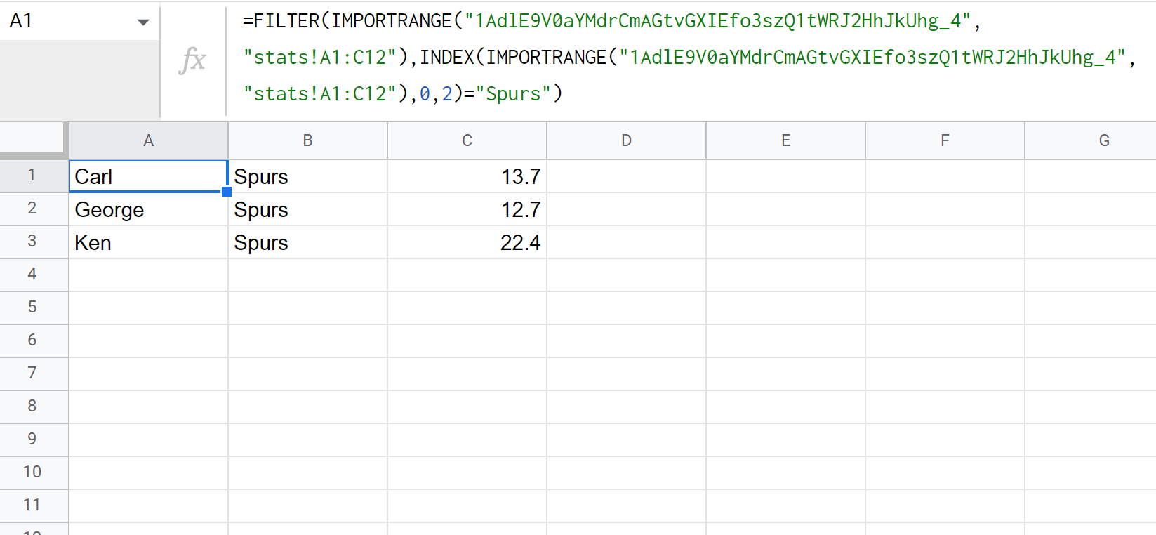
Notice that only the rows where the value in the Team column is equal to “Spurs” were imported.
To filter the rows where the Team column is equal to a different name, simply replace “Spurs” with a different team name in the formula.
Additional Resources
The following tutorials explain how to perform other common tasks in Google Sheets:
Google Sheets: Use IMPORTRANGE with Multiple Sheets
Google Sheets: How to Use IMPORTRANGE with Conditions
Google Sheets: How to Use VLOOKUP From Another Workbook