How to Perform Quantile Regression in Stata

Linear regression is a method we can use to understand the relationship between one or more explanatory variables and a response variable.

Typically when we perform linear regression, we’re interested in estimating the mean value of the response variable based on the value of the explanatory variable. But we could instead estimate the median, or the 0.25 percentile, or the 0.90 percentile, or any percentile we’d like.

This is where quantile regression comes into play. Similar to ordinary linear regression, quantile regression creates a regression equation that predicts some value (e.g. the median, 0.25 percentile, 0.90 percentile, etc.) for a response variable based on the value of the explanatory variable.

This tutorial explains how to perform quantile regression in Stata.

Example: Quantile Regression in Stata

For this example we will use the built-in Stata dataset called auto. First we’ll fit a linear regression model using weight as a predictor variable and mpg as a response variable. This will tell us the expected average mpg of a car, based on its weight. Then we’ll fit a quantile regression model to predict the 0.90 percentile of mpg of a car, based on its weight.

Step 1: Load and view the data.

Use the following command to load the data:

sysuse auto

Use the following command to get a summary of the variables mpg and weight:

summarize mpg weight

Step 2: Perform a simple linear regression.

Use the following command to perform simple linear regression, using weight as the explanatory variable and mpg as the response variable:

regress mpg weight

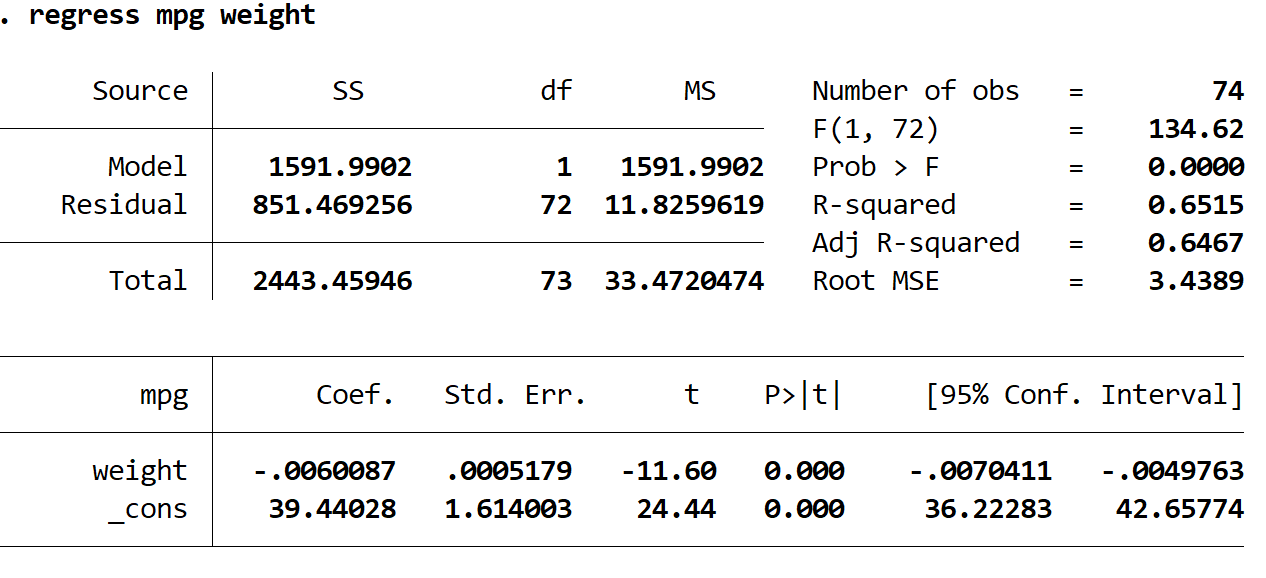
From the output table we can see that the estimated regression equation is:

predicted mpg = 39.44028 – 0.0060087*(weight)

We can use this equation to find the estimated average mpg for a car, given its weight. For example, a car that weighs 4,000 pounds is estimated to have mpg of 15.405:

predicted mpg = 39.44028 – 0.0060087*(4000) = 15.405

Step 3: Perform quantile regression.

Next, let’s perform quantile regression to get the estimated 90^th percentile of a car’s mpg, based on its weight.

Use the qreg command along with quantile(0.90) to perform this quantile regression:

qreg mpg weight, quantile(0.90)

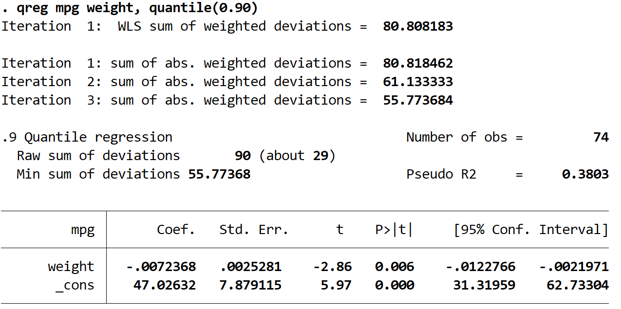
From the output table we can see that the estimated regression equation is:

predicted 90^th percentile of mpg = 47.02632 – 0.0072368*(weight)

We can use this equation to find the estimated mpg for a car in the 90^th percentile, given its weight. For example, the 90^th percentile of mpg for a car that weighs 4,000 pounds is estimated to be 18.709:

predicted 90^th percentile of mpg = 47.02632 – 0.0072368*(4000) = 18.079

Recall that our previous linear regression model told us that a car that weighs 4,000 pounds has an estimated average mpg of 15.405. Thus, it makes sense that this quantile regression model tells us that a car that weighs 4,000 pounds would need an mpg of 18.079 to be in the 90^th percentile of all cars with that particular weight.

Multiple Quantile Regressions at Once in Stata

It’s also possible to perform multiple quantile regressions at once in Stata. For example, suppose we are interested in estimating the 25^th percentile, the median (e.g. 50^th percentile), and the 90^th percentile all at once.

To do so, we can use the sqreg command along with the q() command to specify which quantiles to estimate:

sqreg mpg weight, q(0.25, 0.50, 0.90)

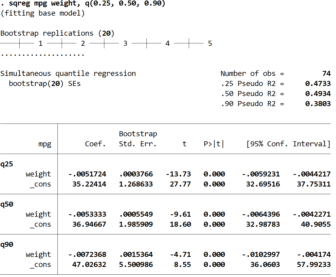
Using this output, we can construct the estimated regression equations for each quantile regression:

(1) predicted 25^th percentile of mpg = 35.22414 – 0.0051724*(weight)

(2) predicted 50^th percentile of mpg = 36.94667 – 0.0053333*(weight)

(3) predicted 90^th percentile of mpg = 47.02632 – 0.0072368*(weight)

Additional Resources

How to Perform Simple Linear Regression in Stata
How to Perform Multiple Linear Regression in Stata
How to Perform Quadratic Regression in Stata