“Statistical significance is the least interesting thing about the results. You should describe the results in terms of measures of magnitude – not just, does a treatment affect people, but how much does it affect them.” -Gene V. Glass
In statistics, we often use p-values to determine if there is a statistically significant difference between two groups.
For example, suppose we want to know if two different studying techniques lead to different test scores. So, we have one group of 20 students use one studying technique to prepare for a test while another group of 20 students uses a different studying technique. We then have each student take the same test.
After running a two-sample t-test for a difference in means, we find that the p-value of the test is 0.001. If we use a 0.05 significance level, then this means there is a statistically significant difference between the mean test scores of the two groups. Thus, studying technique has an impact on test scores.
However, while the p-value tells us that studying technique has an impact on test scores, it doesn’t tell us the size of the impact. To understand this, we need to know the effect size.
What is Effect Size?
An effect size is a way to quantify the difference between two groups.
While a p-value can tell us whether or not there is a statistically significant difference between two groups, an effect size can tell us how large this difference actually is. In practice, effect sizes are much more interesting and useful to know than p-values.
There are three ways to measure effect size, depending on the type of analysis you’re doing:
1. Standardized Mean Difference
When you’re interested in studying the mean difference between two groups, the appropriate way to calculate the effect size is through a standardized mean difference. The most popular formula to use is known as Cohen’s d, which is calculated as:
Cohen’s d = (x1 – x2) / s
where x1 and x2 are the sample means of group 1 and group 2, respectively, and s is the standard deviation of the population from which the two groups were taken.
Using this formula, the effect size is easy to interpret:
- A d of 1 indicates that the two group means differ by one standard deviation.
- A d of 2 means that the group means differ by two standard deviations.
- A d of 2.5 indicates that the two means differ by 2.5 standard deviations, and so on.
Another way to interpret the effect size is as follows: An effect size of 0.3 means the score of the average person in group 2 is 0.3 standard deviations above the average person in group 1 and thus exceeds the scores of 62% of those in group 1.
The following table shows various effect sizes and their corresponding percentiles:
| Effect Size | Percentage of Group 2 who would be below average person in Group 1 |
|---|---|
| 0.0 | 50% |
| 0.2 | 58% |
| 0.4 | 66% |
| 0.6 | 73% |
| 0.8 | 79% |
| 1.0 | 84% |
| 1.2 | 88% |
| 1.4 | 92% |
| 1.6 | 95% |
| 1.8 | 96% |
| 2.0 | 98% |
| 2.5 | 99% |
| 3.0 | 99.9% |
The larger the effect size, the larger the difference between the average individual in each group.
In general, a d of 0.2 or smaller is considered to be a small effect size, a d of around 0.5 is considered to be a medium effect size, and a d of 0.8 or larger is considered to be a large effect size.
Thus, if the means of two groups don’t differ by at least 0.2 standard deviations, the difference is trivial, even if the p-value is statistically significant.
2. Correlation Coefficient
When you’re interested in studying the quantitative relationship between two variables, the most popular way to calculate the effect size is through the Pearson Correlation Coefficient. This is a measure of the linear association between two variables X and Y. It has a value between -1 and 1 where:
- -1 indicates a perfectly negative linear correlation between two variables
- 0 indicates no linear correlation between two variables
- 1 indicates a perfectly positive linear correlation between two variables
The formula to calculate the Pearson Correlation Coefficient is quite complex, but it can be found here for those who are interested.
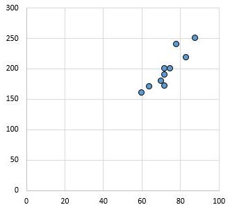
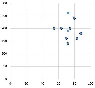
The further away the correlation coefficient is from zero, the stronger the linear relationship between two variables. This can also be seen by creating a simple scatterplot of the values for variables X and Y.
For example, the following scatterplot shows the values of two variables that have a correlation coefficient of r = 0.94.
This value is far from zero, which indicates that there is a strong positive relationship between the two variables.

Conversely, the following scatterplot shows the values of two variables that have a correlation coefficient of r = 0.03. This value is close to zero, which indicates that there is virtually no relationship between the two variables.

In general, the effect size is considered to be low if the value of the Pearson Correlation Coefficient r is around 0.1, medium if r is around 0.3, and large if r is 0.5 or greater.
3. Odds Ratio
When you’re interested in studying the odds of success in a treatment group relative to the odds of success in a control group, the most popular way to calculate the effect size is through the odds ratio.
For example, suppose we have the following table:
| Effect Size | # Successes | # Failures |
|---|---|---|
| Treatment Group | A | B |
| Control Group | C | D |
The odds ratio would be calculated as:
Odds ratio = (AD) / (BC)
The further away the odds ratio is from 1, the higher the likelihood that the treatment has an actual effect.
The Advantages of Using Effect Sizes Over P-Values
Effect sizes have several advantages over p-values:
1. An effect size helps us get a better idea of how large the difference is between two groups or how strong the association is between two groups. A p-value can only tell us whether or not there is some significant difference or some significant association.
2. Unlike p-values, effect sizes can be used to quantitatively compare the results of different studies done in different settings. For this reason, effect sizes are often used in meta-analyses.
3. P-values can be affected by large sample sizes. The larger the sample size, the greater the statistical power of a hypothesis test, which enables it to detect even small effects. This can lead to low p-values, despite small effect sizes that may have no practical significance.
A simple example can make this clear: Suppose we want to know whether two studying techniques lead to different test scores. We have one group of 20 students use one studying technique while another group of 20 students uses a different studying technique. We then have each student take the same test.
The mean score for group 1 is 90.65 and the mean score for group 2 is 90.75. The standard deviation for sample 1 is 2.77 and the standard deviation for sample 2 is 2.78.
When we perform an independent two-sample t test, it turns out that the test statistic is -0.113 and the corresponding p-value is 0.91. The difference between the mean test scores is not statistically significant.
However, consider if the sample sizes of the two samples were both 200, yet the means and the standard deviations remained the exact same.
In this case, an independent two-sample t test would reveal that the test statistic is -1.97 and the corresponding p-value is just under 0.05. The difference between the mean test scores is statistically significant.
The underlying reason that large sample sizes can lead to statistically significant conclusions is due to the formula used to calculate the test statistics t:
test statistic t = [ (x1 – x2) – d ] / (√s21 / n1 + s22 / n2)
Notice that when n1 and n2 are small, the entire denominator of the test statistic t is small. And when we divide by a small number, we end up with a large number. This means the test statistic t will be large and the corresponding p-value will be small, thus leading to statistically significant results.
What is Considered a Good Effect Size?
One question students often have is: What is considered a good effect size?
The short answer: An effect size can’t be “good” or “bad” since it simply measures the size of the difference between two groups or the strength of the association between two two groups.
However, we can use the following rules of thumb to quantify whether an effect size is small, medium or large:
Cohen’s D:
- A d of 0.2 or smaller is considered to be a small effect size.
- A d of 0.5 is considered to be a medium effect size.
- A d of 0.8 or larger is considered to be a large effect size.
Pearson Correlation Coefficient
- An absolute value of r around 0.1 is considered a low effect size.
- An absolute value of r around 0.3 is considered a medium effect size.
- An absolute value of r greater than .5 is considered to be a large effect size.
However, the definition of a “strong” correlation can vary from one field to the next. Refer to this article to gain a better understanding of what is considered a strong correlation in different industries.