A Kruskal-Wallis Test is used to determine whether or not there is a statistically significant difference between the medians of three or more independent groups. It is considered to be the non-parametric equivalent of the One-Way ANOVA.
This tutorial explains how to conduct a Kruskal-Wallis Test in Stata.
How to Perform a Kruskal-Wallis Test in Stata
For this example we will use the census dataset, which contains 1980 census data for all fifty states in the U.S. Within the dataset, the states are classified into four different regions:
- Northeast
- North Central
- South
- West
We will perform a Kruskal-Wallis Test to determine if the median age is equal across these four regions.
Step 1: Load and view the data.
First, load the dataset by typing the following command into the Command box:
use http://www.stata-press.com/data/r13/census
Get a quick summary of the dataset by using the following command:
summarize
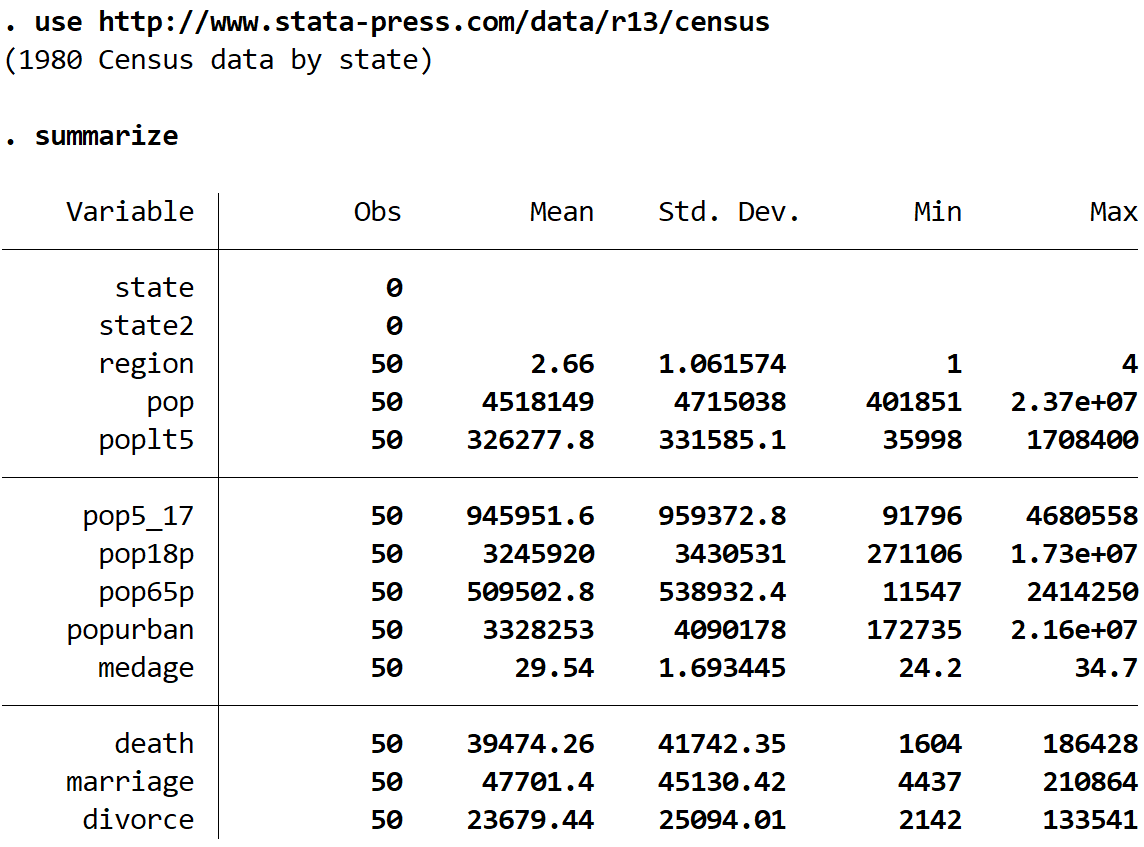
We can see that there are 13 different variables in this dataset, but the only two we will be working with are medage (median age) and region.
Step 2: Visualize the data.
Before we perform the Kruskal-Wallis Test, let’s first create some box plots to visualize the distribution of median age for each of the four regions:
graph box medage, over(region)
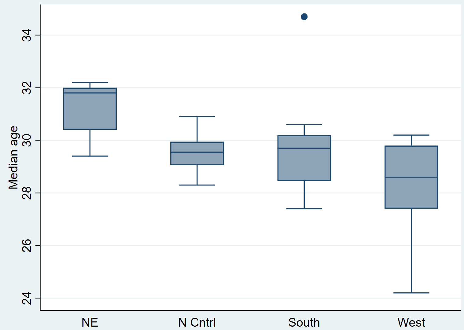
Just from looking at the box plots we can see that the distributions seem to vary between regions. Next, we’ll perform a Kruskal-Wallis Test to see if these differences are statistically significant.
Step 3: Perform a Kruskal-Wallis Test.
Use the following syntax to perform a Kruskal-Wallis Test:
kwallis measurement_variable, by(grouping_variable)
In our case, we will use the following syntax:
kwallis medage, by(region)
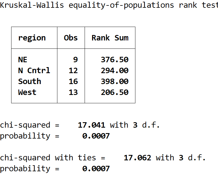
Here is how to interpret the output:
Summary table: This table shows the number of observations per region and the rank sums for each region.
Chi-squared with ties: This is the value of the test statistic, which turns out to be 17.062.
probability: This is the p-value that corresponds to the test statistic, which turns out to be 0.0007. Since this value is less than .05, we can reject the null hypothesis and conclude that the median age is not equal across the four regions.
Step 4: Report the results.
Lastly, we want to report the results of the Kruskal-Wallis Test. Here is an example of how to do so:
A Kruskal-Wallist Test was performed to determine if the median age of individuals was the same across the following four regions in the United States:
- Northeast (n = 9)
- North Central (n = 12)
- South (n = 16)
- West (n = 13)
The test revealed that the median age of individuals was not the same (X2 =17.062, p = 0.0007) across the four regions. That is, there was a statistically significant difference in median age between two or more of the regions.