Multivariate Adaptive Regression Splines in R

---

Multivariate adaptive regression splines (MARS) can be used to model nonlinear relationships between a set of predictor variables and a response variable.

This method works as follows:

1. Divide a dataset into k pieces.

2. Fit a regression model to each piece.

3. Use k-fold cross-validation to choose a value for k.

This tutorial provides a step-by-step example of how to fit a MARS model to a dataset in R.

Step 1: Load Necessary Packages

For this example we’ll use the Wage dataset from the ISLR package, which contains the annual wages for 3,000 individuals along with a variety of predictor variables like age, education, race, and more.

Before we fit a MARS model to the data, we’ll load the necessary packages:

library(ISLR)      #contains Wage dataset
library(dplyr)     #data wrangling
library(ggplot2)   #plotting
library(earth)     #fitting MARS models
library(caret)     #tuning model parameters

Step 2: View Data

Next, we’ll view the first six rows of the dataset we’re working with:

#view first six rows of data
head(Wage)

       year age           maritl     race       education             region
231655 2006  18 1. Never Married 1. White    1. =Very Good 2. No       4.255273     70.47602
161300  1. Industrial      1. =Very Good 1. Yes      5.041393     154.68529
11443   2. Information     1. =Very Good 1. Yes      4.845098     127.11574

Step 3: Build & Optimize the MARS Model

Next, we’ll build the MARS model for this dataset and perform k-fold cross-validation to determine which model produces the lowest test RMSE (root mean squared error).

#create a tuning grid
hyper_grid grid(degree = 1:3,
                          nprune = seq(2, 50, length.out = 10) %>%
                          floor())

#make this example reproducible
set.seed(1)

#fit MARS model using k-fold cross-validation
cv_mars earth",
  metric = "RMSE",
  trControl = trainControl(method = "cv", number = 10),
  tuneGrid = hyper_grid)

#display model with lowest test RMSE
cv_mars$results %>%
  filter(nprune==cv_mars$bestTune$nprune, degree =cv_mars$bestTune$degree)    
degree	nprune	RMSE	 Rsquared   MAE	      RMSESD	RsquaredSD   MAESD		
1	12	33.8164  0.3431804  22.97108  2.240394	0.03064269   1.4554

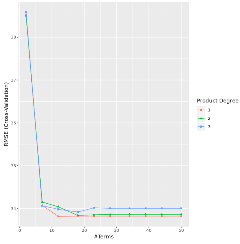
From the output we can see that the model that produced the lowest test MSE was one with only first-order effects (i.e. no interaction terms) and 12 terms. This model produced a root mean squared error (RMSE) of 33.8164.

Note: We used method=”earth” to specify a MARS model. You can find the documentation for this method here.

We can also create a plot to visualize the test RMSE based on the degree and the number of terms:

#display test RMSE by terms and degree
ggplot(cv_mars)

In practice we would fit a MARS model along with several other types of models like:

• Multiple Linear Regression
• Polynomial Regression
• Ridge Regression
• Lasso Regression
• Principal Components Regression
• Partial Least Squares

We would then compare each model to determine which one lead to the lowest test error and choose that model as the optimal one to use.

The complete R code used in this example can be found here.