Polynomial regression is a technique we can use when the relationship between a predictor variable and a response variable is nonlinear.
This type of regression takes the form:
Y = β0 + β1X + β2X2 + … + βhXh + ε
where h is the “degree” of the polynomial.
This tutorial provides a step-by-step example of how to perform polynomial regression in R.
Step 1: Create the Data
For this example we’ll create a dataset that contains the number of hours studied and final exam score for a class of 50 students:
#make this example reproducible
set.seed(1)

#create dataset
df runif(50, 5, 15), score=50)
df$score = df$score + df$hours^3/150 + df$hours*runif(50, 1, 2)

#view first six rows of data
head(data)

      hours    score
1  7.655087 64.30191
2  8.721239 70.65430
3 10.728534 73.66114
4 14.082078 86.14630
5  7.016819 59.81595
6 13.983897 83.60510
Step 2: Visualize the Data
Before we fit a regression model to the data, let’s first create a scatterplot to visualize the relationship between hours studied and exam score:
library(ggplot2)

ggplot(df, aes(x=hours, y=score)) +
  geom_point()

We can see that the data exhibits a bit of a quadratic relationship, which indicates that polynomial regression could fit the data better than simple linear regression.
Step 3: Fit the Polynomial Regression Models
Next, we’ll fit five different polynomial regression models with degrees h = 1…5 and use k-fold cross-validation with k=10 folds to calculate the test MSE for each model:
#randomly shuffle data
df.shuffled sample(nrow(df)),]

#define number of folds to use for k-fold cross-validation
K #define degree of polynomials to fit
degree #create k equal-sized folds
folds seq(1,nrow(df.shuffled)),breaks=K,labels=FALSE)

#create object to hold MSE's of models
mse = matrix(data=NA,nrow=K,ncol=degree)

#Perform K-fold cross validation
for(i in 1:K){

    #define training and testing data
    testIndexes which(folds==i,arr.ind=TRUE)
    testData     #use k-fold cv to evaluate models
    for (j in 1:degree){
        fit.train = lm(score ~ poly(hours,j), data=trainData)
        fit.test = predict(fit.train, newdata=testData)
        mse[i,j] = mean((fit.test-testData$score)^2)
    }
}

#find MSE for each degree
colMeans(mse)

[1]  9.802397  8.748666  9.601865 10.592569 13.545547
From the output we can see the test MSE for each model:
- Test MSE with degree h = 1: 9.80
- Test MSE with degree h = 2: 8.75
- Test MSE with degree h = 3: 9.60
- Test MSE with degree h = 4: 10.59
- Test MSE with degree h = 5: 13.55
The model with the lowest test MSE turned out to be the polynomial regression model with degree h =2.
This matches our intuition from the original scatterplot: A quadratic regression model fits the data best.
Step 4: Analyze the Final Model
Lastly, we can obtain the coefficients of the best performing model:
#fit best model
best = lm(score ~ poly(hours,2, raw=T), data=df)

#view summary of best model
summary(best)

Call:
lm(formula = score ~ poly(hours, 2, raw = T), data = df)

Residuals:
    Min      1Q  Median      3Q     Max
-5.6589 -2.0770 -0.4599  2.5923  4.5122

Coefficients:
                         Estimate Std. Error t value Pr(>|t|)
(Intercept)              54.00526    5.52855   9.768 6.78e-13 ***
poly(hours, 2, raw = T)1 -0.07904    1.15413  -0.068  0.94569
poly(hours, 2, raw = T)2  0.18596    0.05724   3.249  0.00214 **
---
Signif. codes:  0 '***' 0.001 '**' 0.01 '*' 0.05 '.' 0.1 ' ' 1
From the output we can see that the final fitted model is:
Score = 54.00526 – .07904*(hours) + .18596*(hours)2
We can use this equation to estimate the score that a student will receive based on the number of hours they studied.
For example, a student who studies for 10 hours is expected to receive a score of 71.81:
Score = 54.00526 – .07904*(10) + .18596*(10)2 = 71.81
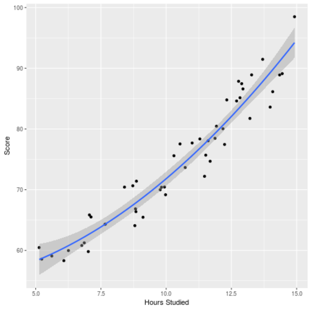
We can also plot the fitted model to see how well it fits the raw data:
ggplot(df, aes(x=hours, y=score)) +
          geom_point() +
          stat_smooth(method='lm', formula = y ~ poly(x,2), size = 1) +
          xlab('Hours Studied') +
          ylab('Score')
You can find the complete R code used in this example here.