Cramer’s V is a measure of the strength of association between two nominal variables.
It ranges from 0 to 1 where:
- 0 indicates no association between the two variables.
- 1 indicates a strong association between the two variables.
It is calculated as:
Cramer’s V = √(X2/n) / min(c-1, r-1)
where:
- X2: The Chi-square statistic
- n: Total sample size
- r: Number of rows
- c: Number of columns
This tutorial provides two examples of how to calculate Cramer’s V for a contingency table in Excel.
Example: Calculating Cramer’s V in Excel
Suppose we would like to understand if there is an association between two exam prep methods and the passing rate of students.
The following table shows the number of students who passed and failed the exam, based on the exam prep method they used:

The following screenshot shows the exact formulas we can use to calculate Cramer’s V for a 2×2 table that contains data for 36 students:
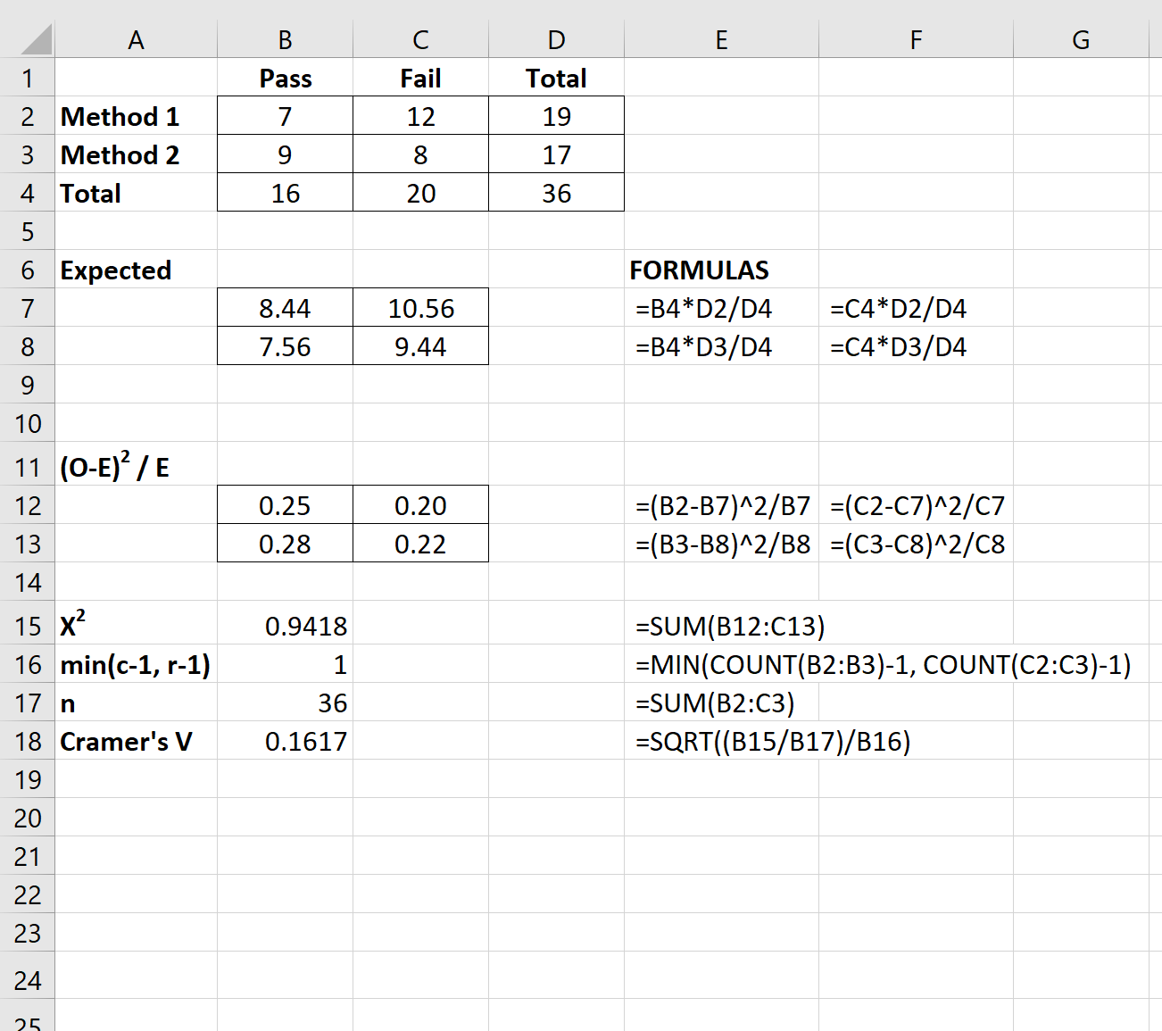
Cramer’s V turns out to be 0.1617.
We can use the following table to determine whether a Cramer’s V should be considered a small, medium, or large effect size based on the degrees of freedom used:

In this example, the degrees of freedom is equal to 1. Thus, a Cramer’s V of 0.1617 would be considered a small effect size.
In other words, there’s a fairly weak association between the exam prep method used and the passing rate of students.
Additional Resources
How to Calculate Cramer’s V in R
How to Calculate Cramer’s V in Python