When the relationship between a set of predictor variables and a response variable is linear, methods like multiple linear regression can produce accurate predictive models.
However, when the relationship between a set of predictors and a response is more complex, then non-linear methods can often produce more accurate models.
One such method is classification and regression trees (CART), which use a set of predictor variable to build decision trees that predict the value of a response variable.
If the response variable is continuous then we can build regression trees and if the response variable is categorical then we can build classification trees.
This tutorial explains how to build both regression and classification trees in R.
Example 1: Building a Regression Tree in R
For this example, we’ll use the Hitters dataset from the ISLR package, which contains various information about 263 professional baseball players.
We will use this dataset to build a regression tree that uses the predictor variables home runs and years played to predict the Salary of a given player.
Use the following steps to build this regression tree.
Step 1: Load the necessary packages.
First, we’ll load the necessary packages for this example:
library(ISLR) #contains Hitters dataset
library(rpart) #for fitting decision trees
library(rpart.plot) #for plotting decision trees
Step 2: Build the initial regression tree.
First, we’ll build a large initial regression tree. We can ensure that the tree is large by using a small value for cp, which stands for “complexity parameter.”
This means we will perform new splits on the regression tree as long as the overall R-squared of the model increases by at least the value specified by cp.
We’ll then use the printcp() function to print the results of the model:
#build the initial tree
tree control(cp=.0001))

#view results
printcp(tree)

Variables actually used in tree construction:
[1] HmRun Years

Root node error: 53319113/263 = 202734

n=263 (59 observations deleted due to missingness)

           CP nsplit rel error  xerror    xstd
1  0.24674996      0   1.00000 1.00756 0.13890
2  0.10806932      1   0.75325 0.76438 0.12828
3  0.01865610      2   0.64518 0.70295 0.12769
4  0.01761100      3   0.62652 0.70339 0.12337
5  0.01747617      4   0.60891 0.70339 0.12337
6  0.01038188      5   0.59144 0.66629 0.11817
7  0.01038065      6   0.58106 0.65697 0.11687
8  0.00731045      8   0.56029 0.67177 0.11913
9  0.00714883      9   0.55298 0.67881 0.11960
10 0.00708618     10   0.54583 0.68034 0.11988
11 0.00516285     12   0.53166 0.68427 0.11997
12 0.00445345     13   0.52650 0.68994 0.11996
13 0.00406069     14   0.52205 0.68988 0.11940
14 0.00264728     15   0.51799 0.68874 0.11916
15 0.00196586     16   0.51534 0.68638 0.12043
16 0.00016686     17   0.51337 0.67577 0.11635
17 0.00010000     18   0.51321 0.67576 0.11615
n=263 (59 observations deleted due to missingness)
Step 3: Prune the tree.
Next, we’ll prune the regression tree to find the optimal value to use for cp (the complexity parameter) that leads to the lowest test error.
Note that the optimal value for cp is the one that leads to the lowest xerror in the previous output, which represents the error on the observations from the cross-validation data.
#identify best cp value to use
best min(tree$cptable[,"xerror"]),"CP"]

#produce a pruned tree based on the best cp value
pruned_tree prune(tree, cp=best)

#plot the pruned tree
prp(pruned_tree,
    faclen=0, #use full names for factor labels
    extra=1, #display number of obs. for each terminal node
    roundint=F, #don't round to integers in output
    digits=5) #display 5 decimal places in output
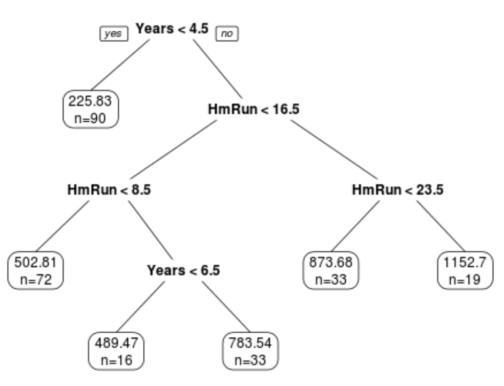
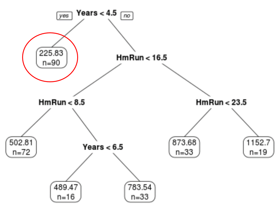
We can see that the final pruned tree has six terminal nodes. Each terminal node shows the predicted salary of player’s in that node along with the number of observations from the original dataset that belong to that note.
For example, we can see that in the original dataset there were 90 players with less than 4.5 years of experience and their average salary was $225.83k.
Step 4: Use the tree to make predictions.
We can use the final pruned tree to predict a given player’s salary based on their years of experience and average home runs.
For example, a player who has 7 years of experience and 4 average home runs has a predicted salary of $502.81k.
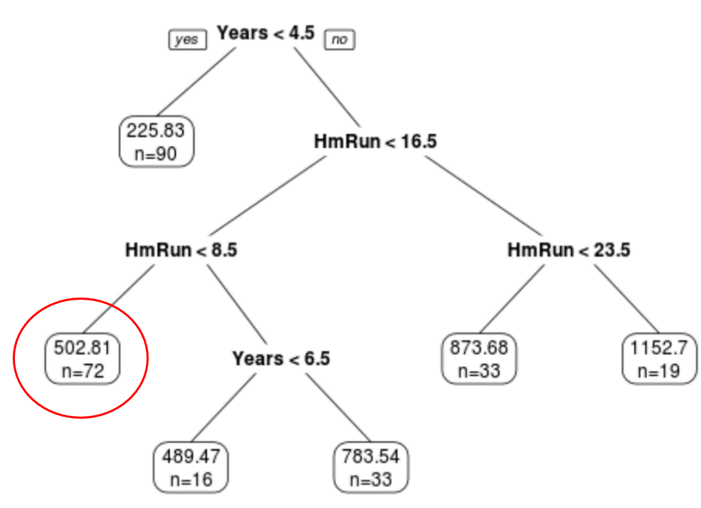
We can use the predict() function in R to confirm this:
#define new player
new #use pruned tree to predict salary of this player
predict(pruned_tree, newdata=new)

502.8079
Example 2: Building a Classification Tree in R
For this example, we’ll use the ptitanic dataset from the rpart.plot package, which contains various information about passengers aboard the Titanic.
We will use this dataset to build a classification tree that uses the predictor variables class, sex, and age to predict whether or not a given passenger survived.
Use the following steps to build this classification tree.
Step 1: Load the necessary packages.
First, we’ll load the necessary packages for this example:
library(rpart) #for fitting decision trees
library(rpart.plot) #for plotting decision trees
Step 2: Build the initial classification tree.
First, we’ll build a large initial classification tree. We can ensure that the tree is large by using a small value for cp, which stands for “complexity parameter.”
This means we will perform new splits on the classification tree as long as the overall fit of the model increases by at least the value specified by cp.
We’ll then use the printcp() function to print the results of the model:
#build the initial tree
tree control(cp=.0001))

#view results
printcp(tree)

Variables actually used in tree construction:
[1] age    pclass sex

Root node error: 500/1309 = 0.38197

n= 1309

      CP nsplit rel error xerror     xstd
1 0.4240      0     1.000  1.000 0.035158
2 0.0140      1     0.576  0.576 0.029976
3 0.0095      3     0.548  0.578 0.030013
4 0.0070      7     0.510  0.552 0.029517
5 0.0050      9     0.496  0.528 0.029035
6 0.0025     11     0.486  0.532 0.029117
7 0.0020     19     0.464  0.536 0.029198
8 0.0001     22     0.458  0.528 0.029035
Step 3: Prune the tree.
Next, we’ll prune the regression tree to find the optimal value to use for cp (the complexity parameter) that leads to the lowest test error.
Note that the optimal value for cp is the one that leads to the lowest xerror in the previous output, which represents the error on the observations from the cross-validation data.
#identify best cp value to use
best min(tree$cptable[,"xerror"]),"CP"]

#produce a pruned tree based on the best cp value
pruned_tree prune(tree, cp=best)

#plot the pruned tree
prp(pruned_tree,
    faclen=0, #use full names for factor labels
    extra=1, #display number of obs. for each terminal node
    roundint=F, #don't round to integers in output
    digits=5) #display 5 decimal places in output
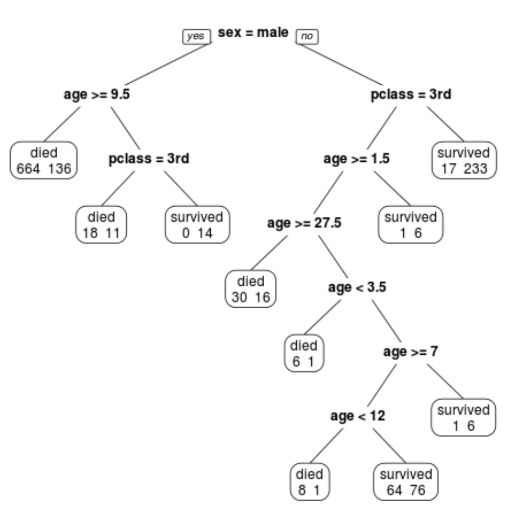
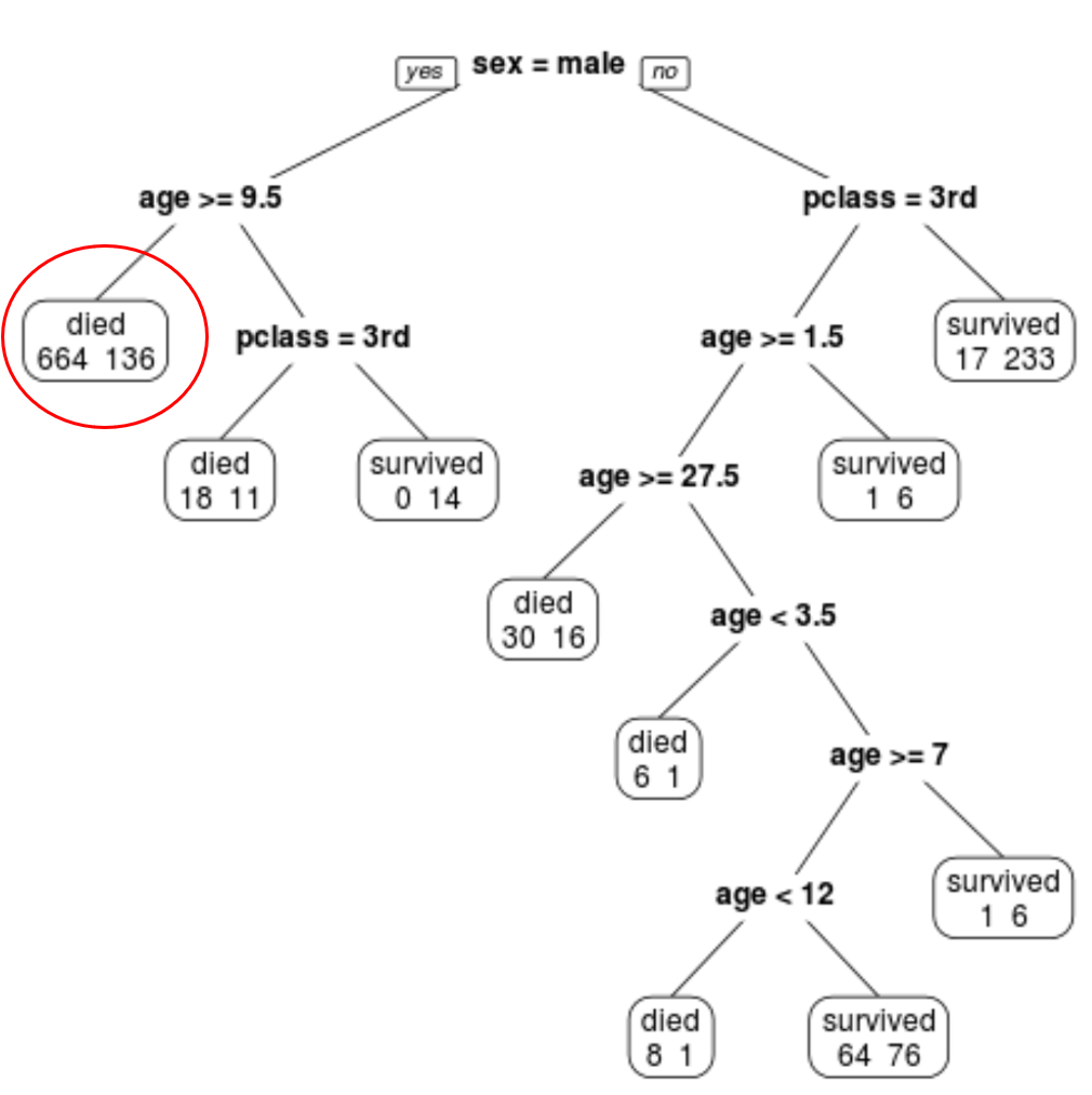
We can see that the final pruned tree has 10 terminal nodes. Each terminal node shows the number of passengers that died along with the number that survived.
For example, in the far left node we see that 664 passengers died and 136 survived.
Step 4: Use the tree to make predictions.
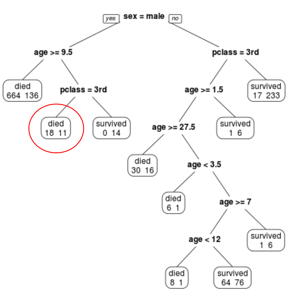
We can use the final pruned tree to predict the probability that a given passenger will survive based on their class, age, and sex.
For example, a male passenger who is in 1st class and is 8 years old has a survival probability of 11/29 = 37.9%.
You can find the complete R code used in these examples here.