When we create a decision tree for a given dataset, we only use one training dataset to build the model.
However, the downside of using a single decision tree is that it tends to suffer from high variance. That is, if we split the dataset into two halves and apply the decision tree to both halves, the results could be quite different.
One method that we can use to reduce the variance of a single decision tree is known as bagging, sometimes referred to as bootstrap aggregating.
Bagging works as follows:
1. Take b bootstrapped samples from the original dataset.
2. Build a decision tree for each bootstrapped sample.
3. Average the predictions of each tree to come up with a final model.
Through building hundreds or even thousands of individual decision trees and taking the average predictions from all of the trees, we often end up with a fitted bagged model that produces a much lower test error rate compared to a single decision tree.
This tutorial provides a step-by-step example of how to create a bagged model in R.
Step 1: Load the Necessary Packages
First, we’ll load the necessary packages for this example:
library(dplyr)       #for data wrangling
library(e1071)       #for calculating variable importance
library(caret)       #for general model fitting
library(rpart)       #for fitting decision trees
library(ipred)       #for fitting bagged decision trees
Step 2: Fit the Bagged Model
For this example, we’ll use a built-in R dataset called airquality which contains air quality measurements in New York on 153 individual days.
#view structure of airquality dataset
str(airquality)

'data.frame':	153 obs. of  6 variables:
 $ Ozone  : int  41 36 12 18 NA 28 23 19 8 NA ...
 $ Solar.R: int  190 118 149 313 NA NA 299 99 19 194 ...
 $ Wind   : num  7.4 8 12.6 11.5 14.3 14.9 8.6 13.8 20.1 8.6 ...
 $ Temp   : int  67 72 74 62 56 66 65 59 61 69 ...
 $ Month  : int  5 5 5 5 5 5 5 5 5 5 ...
 $ Day    : int  1 2 3 4 5 6 7 8 9 10 ...
The following code shows how to fit a bagged model in R using the bagging() function from the ipred library.
#make this example reproducible
set.seed(1)

#fit the bagged model
bag 150,
  coob = TRUE,
  control = rpart.control(minsplit = 2, cp = 0)
)

#display fitted bagged model
bag

Bagging regression trees with 150 bootstrap replications

Call: bagging.data.frame(formula = Ozone ~ ., data = airquality, nbagg = 150,
    coob = TRUE, control = rpart.control(minsplit = 2, cp = 0))

Out-of-bag estimate of root mean squared error:  17.4973
Note that we chose to use 150 bootstrapped samples to build the bagged model and we specified coob to be TRUE to obtain the estimated out-of-bag error.
We also used the following specifications in the rpart.control() function:
- minsplit = 2: This tells the model to only require 2 observations in a node to split.
- cp = 0. This is the complexity parameter. By setting it to 0, we don’t require the model to be able to improve the overall fit by any amount in order to perform a split.
Essentially these two arguments allow the individual trees to grow extremely deep, which leads to trees with high variance but low bias. Then when we apply bagging we’re able to reduce the variance of the final model while keeping the bias low.
From the output of the model we can see that the out-of-bag estimated RMSE is 17.4973. This is the average difference between the predicted value for Ozone and the actual observed value.
Step 3: Visualize the Importance of the Predictors
Although bagged models tend to provide more accurate predictions compared to individual decision trees, it’s difficult to interpret and visualize the results of fitted bagged models.
We can, however, visualize the importance of the predictor variables by calculating the total reduction in RSS (residual sum of squares) due to the split over a given predictor, averaged over all of the trees. The larger the value, the more important the predictor.
The following code shows how to create a variable importance plot for the fitted bagged model, using the varImp() function from the caret library:
#calculate variable importance
VI names(airquality[,-1]), imp=varImp(bag))

#sort variable importance descending
VI_plot order(VI$Overall, decreasing=TRUE),]

#visualize variable importance with horizontal bar plot
barplot(VI_plot$Overall,
        names.arg=rownames(VI_plot),
        horiz=TRUE,
        col='steelblue',
        xlab='Variable Importance')
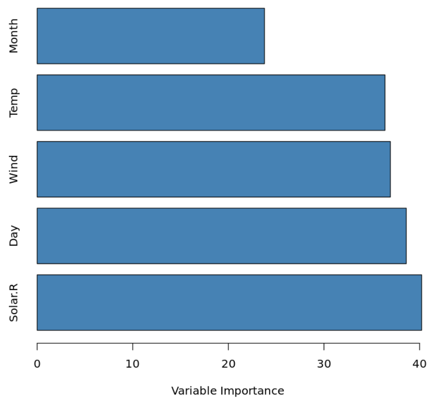
We can see that Solar.R is the most importance predictor variable in the model while Month is the least important.
Step 4: Use the Model to Make Predictions
Lastly, we can use the fitted bagged model to make predictions on new observations.
#define new observation
new #use fitted bagged model to predict Ozone value of new observation
predict(bag, newdata=new)

24.4866666666667
Based on the values of the predictor variables, the fitted bagged model predicts that the Ozone value will be 24.487 on this particular day.
The complete R code used in this example can be found here.