Simple linear regression is a method you can use to understand the relationship between an explanatory variable, x, and a response variable, y.
This tutorial explains how to perform simple linear regression in Stata.
Example: Simple Linear Regression in Stata
Suppose we are interested in understanding the relationship between the weight of a car and its miles per gallon. To explore this relationship, we can perform simple linear regression using weight as an explanatory variable and miles per gallon as a response variable.
Perform the following steps in Stata to conduct a simple linear regression using the dataset called auto, which contains data on 74 different cars.
Step 1: Load the data.
Load the data by typing the following into the Command box:
use http://www.stata-press.com/data/r13/auto
Step 2: Get a summary of the data.
Gain a quick understanding of the data you’re working with by typing the following into the Command box:
summarize
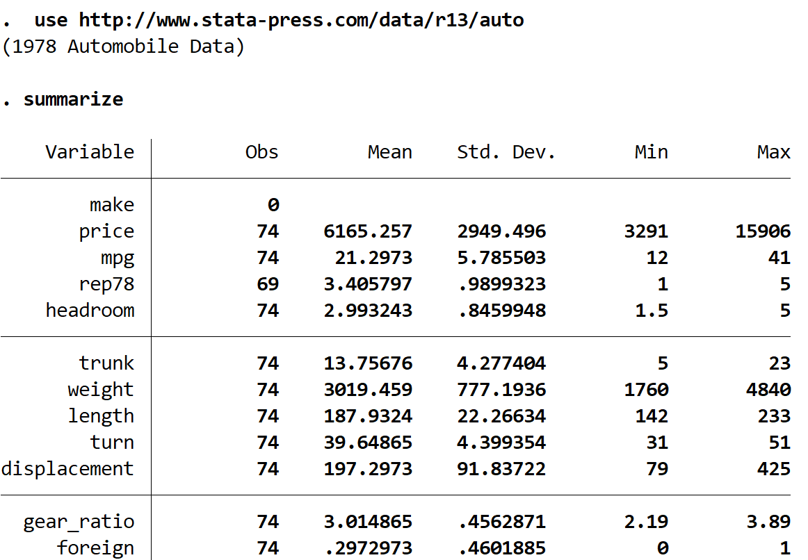
We can see that there are 12 different variables in the dataset, but the only two that we care about are mpg and weight.
Step 3: Visualize the data.
Before we perform simple linear regression, let’s first create a scatterplot of weight vs. mpg so we can visualize the relationship between these two variables and check for any obvious outliers. Type the following into the Command box to create a scatterplot:
scatter mpg weight
This produces the following scatterplot:
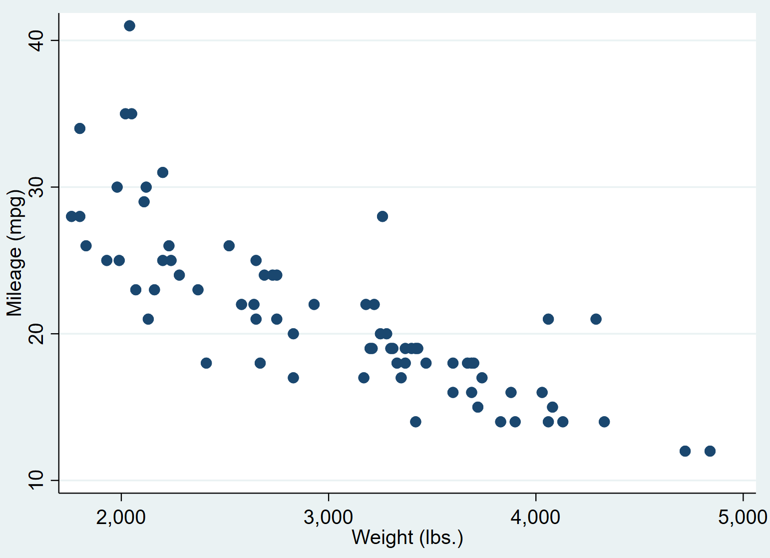
We can see that cars with higher weights tend to have lower miles per gallon. To quantify this relationship, we will now perform a simple linear regression.
Step 4: Perform simple linear regression.
Type the following into the Command box to perform a simple linear regression using weight as an explanatory variable and mpg as a response variable.
regress mpg weight
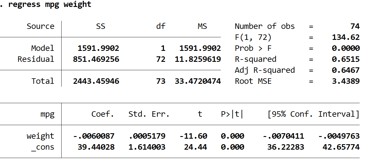
Here is how to interpret the most interesting numbers in the output:
R-squared: 0.6515. This is the proportion of the variance in the response variable that can be explained by the explanatory variable. In this example, 65.15% of the variation in mpg can be explained by weight.
Coef (weight): -0.006. This tells us the average change in the response variable associated with a one unit increase in the explanatory variable. In this example, each one pound increase in weight is associated with a decrease of 0.006 in mpg, on average.
Coef (_cons): 39.44028. This tells us the average value of the response variable when the explanatory variable is zero. In this example, the average mpg is 39.44028 when the weight of a car is zero. This doesn’t actually make much sense to interpret since the weight of a car can’t be zero, but the number 39.44028 is needed to form a regression equation.
P>|t| (weight): 0.000. This is the p-value associated with the test statistic for weight. In this case, since this value is less than 0.05, we can conclude that there is a statistically significant relationship between weight and mpg.
Regression Equation: Lastly, we can form a regression equation using the two coefficient values. In this case, the equation would be:
predicted mpg = 39.44028 – 0.0060087*(weight)
We can use this equation to find the predicted mpg for a car, given its weight. For example, a car that weighs 4,000 pounds is predicted to have mpg of 15.405:
predicted mpg = 39.44028 – 0.0060087*(4000) = 15.405
Step 5: Report the results.
Lastly, we want to report the results of our simple linear regression. Here is an example of how to do so:
A linear regression was performed to quantify the relationship between the weight of a car and its miles per gallon. A sample of 74 cars was used in the analysis.
Results showed that there was a statistically significant relationship between weight and mpg (t = -11.60, p
The regression equation was found to be:
predicted mpg = 39.44 – 0.006(weight)
Each additional pound was associated with a decrease, on average, of -.006 miles per gallon.