Multiple linear regression is a method we can use to understand the relationship between two or more explanatory variables and a response variable.
This tutorial explains how to perform multiple linear regression in Excel.
Note: If you only have one explanatory variable, you should instead perform simple linear regression.
Example: Multiple Linear Regression in Excel
Suppose we want to know if the number of hours spent studying and the number of prep exams taken affects the score that a student receives on a certain college entrance exam.
To explore this relationship, we can perform multiple linear regression using hours studied and prep exams taken as explanatory variables and exam score as a response variable.
Perform the following steps in Excel to conduct a multiple linear regression.
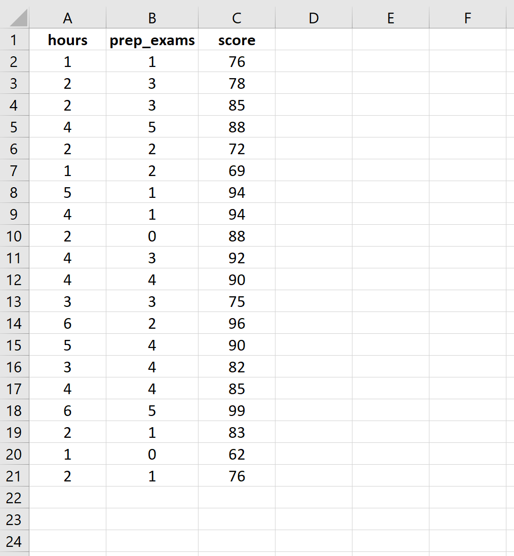
Step 1: Enter the data.
Enter the following data for the number of hours studied, prep exams taken, and exam score received for 20 students:
Step 2: Perform multiple linear regression.
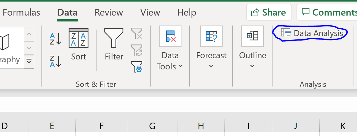
Along the top ribbon in Excel, go to the Data tab and click on Data Analysis. If you don’t see this option, then you need to first install the free Analysis ToolPak.
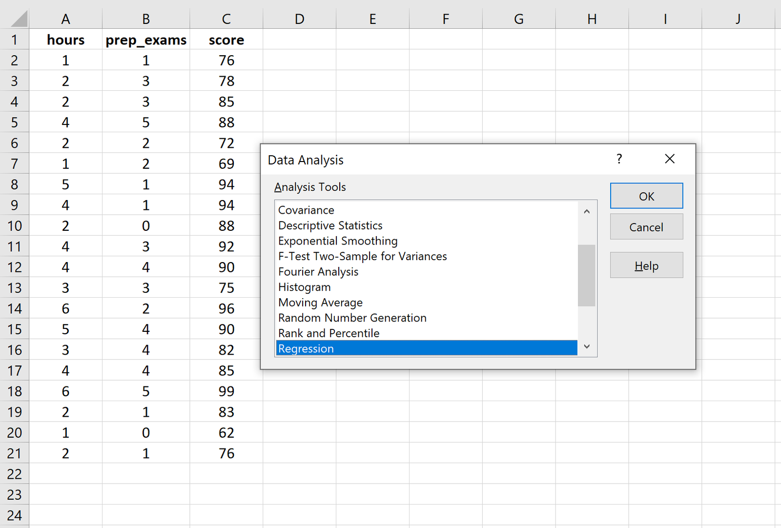
Once you click on Data Analysis, a new window will pop up. Select Regression and click OK.
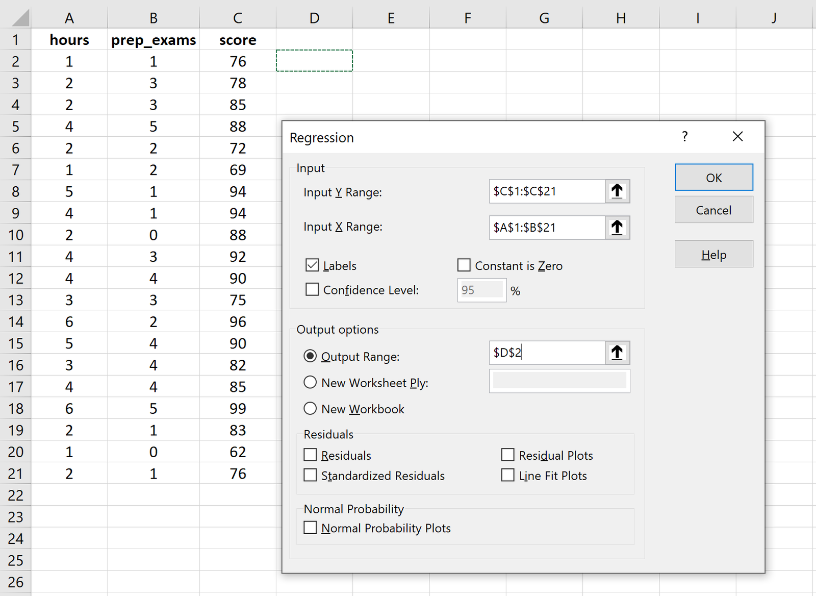
For Input Y Range, fill in the array of values for the response variable. For Input X Range, fill in the array of values for the two explanatory variables. Check the box next to Labels so Excel knows that we included the variable names in the input ranges. For Output Range, select a cell where you would like the output of the regression to appear. Then click OK.
The following output will automatically appear:
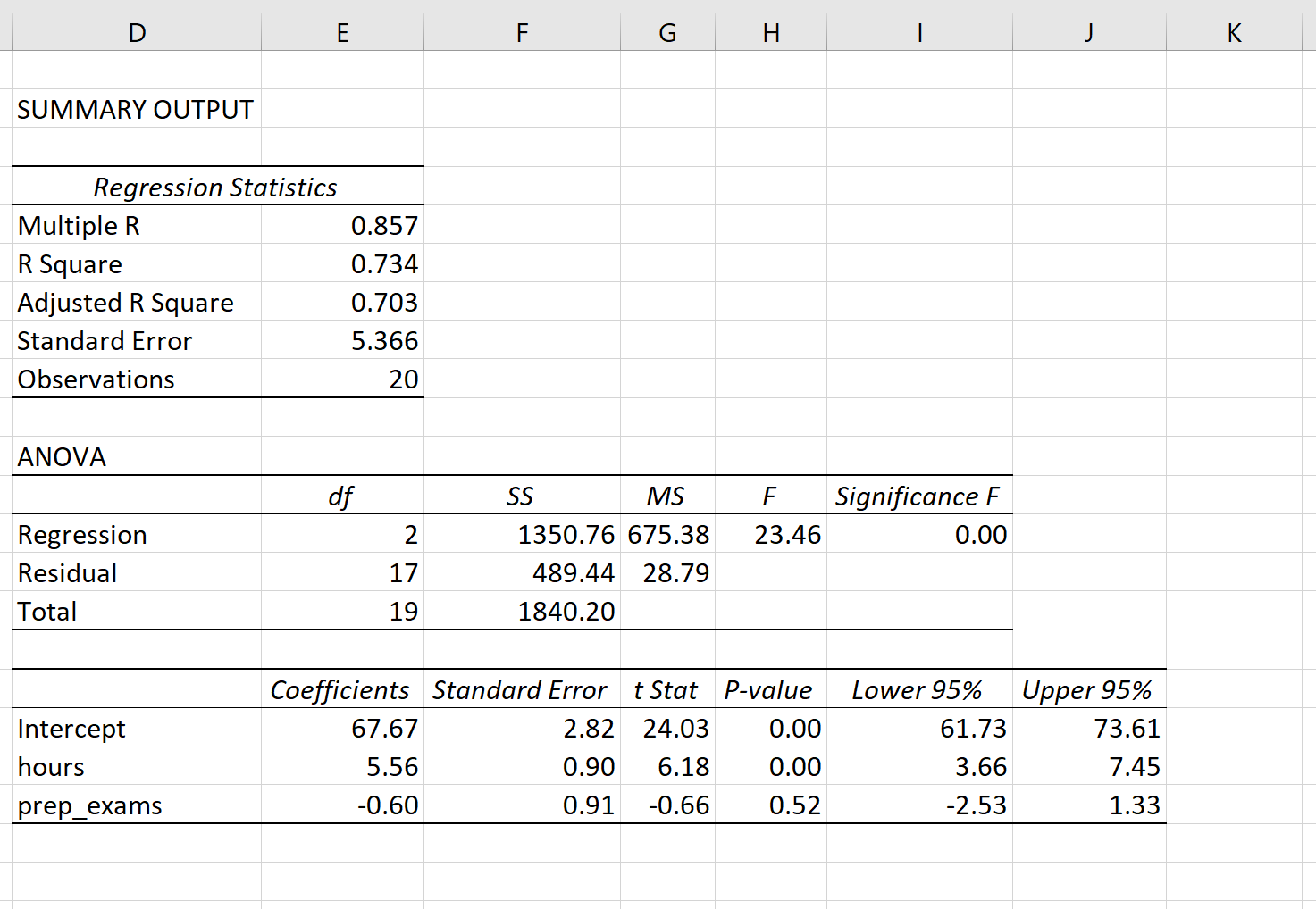
Step 3: Interpret the output.
Here is how to interpret the most relevant numbers in the output:
R Square: 0.734. This is known as the coefficient of determination. It is the proportion of the variance in the response variable that can be explained by the explanatory variables. In this example, 73.4% of the variation in the exam scores can be explained by the number of hours studied and the number of prep exams taken.
Standard error: 5.366. This is the average distance that the observed values fall from the regression line. In this example, the observed values fall an average of 5.366 units from the regression line.
F: 23.46. This is the overall F statistic for the regression model, calculated as regression MS / residual MS.
Significance F: 0.0000. This is the p-value associated with the overall F statistic. It tells us whether or not the regression model as a whole is statistically significant. In other words, it tells us if the two explanatory variables combined have a statistically significant association with the response variable. In this case the p-value is less than 0.05, which indicates that the explanatory variables hours studied and prep exams taken combined have a statistically significant association with exam score.
P-values. The individual p-values tell us whether or not each explanatory variable is statistically significant. We can see that hours studied is statistically significant (p = 0.00) while prep exams taken (p = 0.52) is not statistically signifciant at α = 0.05. Since prep exams taken is not statistically significant, we may end up deciding to remove it from the model.
Coefficients: The coefficients for each explanatory variable tell us the average expected change in the response variable, assuming the other explanatory variable remains constant. For example, for each additional hour spent studying, the average exam score is expected to increase by 5.56, assuming that prep exams taken remains constant.
Here’s another way to think about this: If student A and student B both take the same amount of prep exams but student A studies for one hour more, then student A is expected to earn a score that is 5.56 points higher than student B.
We interpret the coefficient for the intercept to mean that the expected exam score for a student who studies zero hours and takes zero prep exams is 67.67.
Estimated regression equation: We can use the coefficients from the output of the model to create the following estimated regression equation:
exam score = 67.67 + 5.56*(hours) – 0.60*(prep exams)
We can use this estimated regression equation to calculate the expected exam score for a student, based on the number of hours they study and the number of prep exams they take. For example, a student who studies for three hours and takes one prep exam is expected to receive a score of 83.75:
exam score = 67.67 + 5.56*(3) – 0.60*(1) = 83.75
Keep in mind that because prep exams taken was not statistically significant (p = 0.52), we may decide to remove it because it doesn’t add any improvement to the overall model. In this case, we could perform simple linear regression using only hours studied as the explanatory variable.
The results of this simple linear regression analysis can be found here.
Additional Resources
Once you perform multiple linear regression, there are several assumptions you may want to check including:
1. Testing for multicollinearity using VIF.
2. Testing for heterodscedasticity using a Breusch-Pagan test.