This tutorial explains how to perform a reverse VLOOKUP in Google Sheets.
Example: Reverse VLOOKUP in Google Sheets
Suppose we have the following dataset that shows the number of points scored by various basketball teams:

We can use the following VLOOKUP formula to find the number of points associated with the “Knicks” team:
=VLOOKUP("Knicks", A1:B9, 2)
Here’s what this formula does:
- It identifies Knicks as the value to find.
- It specifies A1:B9 as the range to analyze.
- It specifies that we’d like to return the value in the 2nd column from the left.
Here’s how to use this formula in practice:
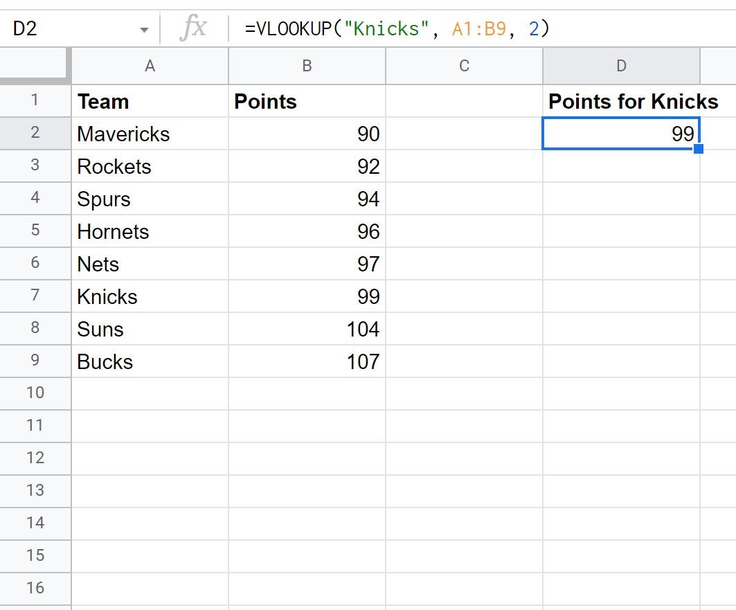
This formula correctly returns the value of 99.
However, suppose we instead want to know which team is associated with a points value of 99.
We can use the following reverse VLOOKUP formula:
=VLOOKUP(99, {B2:B9, A2:A9}, 2)
Here’s what this formula does:
- It identifies 99 as the value to find.
- It specifies B2:B9 and A2:A9 as the ranges to analyze.
- It specifies that we’d like to return the value in the 2nd column from the right.
Here’s how to use this formula in practice:
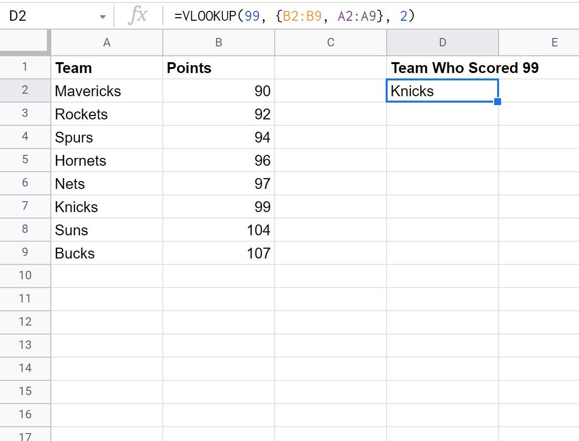
The formula correctly identifies the Knicks as the team with a points value of 99.
Additional Resources
The following tutorials explain how to perform other common operations in Google Sheets:
How to Use a Case Sensitive VLOOKUP in Google Sheets
How to Count Cells with Text in Google Sheets
How to Replace Text in Google Sheets
How to Filter for Cells that Contain Text in Google Sheets