You can use the following basic formula to perform a case sensitive VLOOKUP in Google Sheets:
=INDEX(B2:B10, MATCH(TRUE, EXACT(G2, A2:A10), 0))
This particular formula finds the exact value in cell G2 in the range A2:A10 and returns the corresponding value in the range B2:B10.
The following example shows how to use this formula in practice.
Example: Case Sensitive VLOOKUP in Google Sheets
Suppose we have the following dataset that shows the number of sales made by various salesmen at a company:
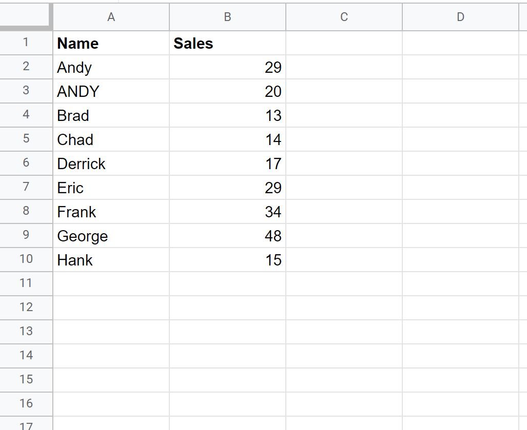
Now suppose we attempt to use the following VLOOKUP formula to look up “Andy” and return his number of sales:
=VLOOKUP(D2, A2:B10, 2)
This formula incorrectly returns the number of sales for ANDY instead of Andy:

Instead, we need to use the following formula that can perform a case-sensitive VLOOKUP:
=INDEX(B2:B10, MATCH(TRUE, EXACT(G2, A2:A10), 0))
This formula correctly returns the number of sales for Andy, which turns out to be 29:
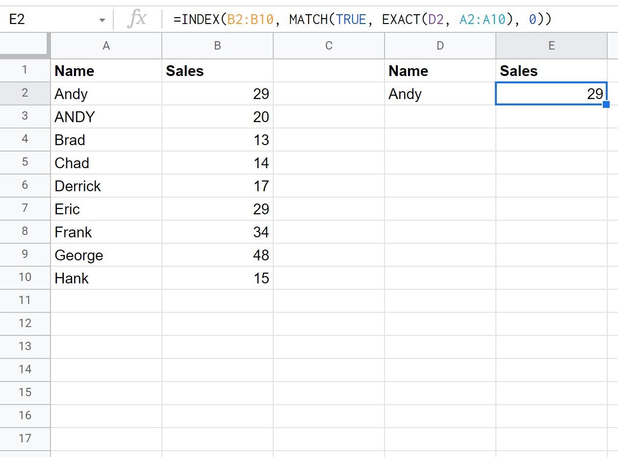
The formula correctly returns the number of sales for Andy instead of ANDY.
Additional Resources
The following tutorials explain how to perform other common operations in Google Sheets:
How to Count Cells with Text in Google Sheets
How to Replace Text in Google Sheets
How to Filter for Cells that Contain Text in Google Sheets