Often you may want to apply conditional formatting to cells that contain specific text in Excel.
The following example shows exactly how to do so.
Example: Conditional Formatting if Cell Contains Text
Suppose we have the following dataset that shows the names of various basketball teams:

Suppose we would like to highlight each team name equal to “Mavs” in column A.
To do so, highlight the values in the range A2:A14, then click the Conditional Formatting icon on the Home tab, then click New Rule:

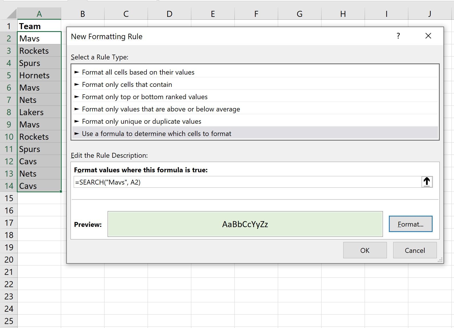
In the new window that appears, click Use a formula to determine which cells to format, then type in the following formula into the box:
=SEARCH("Mavs", A2)
Then click the Format button and choose a color to use to fill in the cells that contain “Mavs” in the name. Then click OK:

Each team that contains “Mavs” in the name will automatically be highlighted:

Note that you can also highlight cells that contain partial text by using the asterisk (*) wildcard with the SEARCH function.
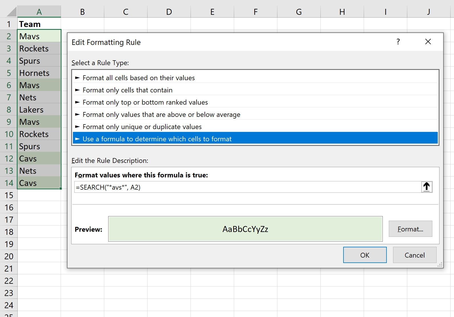
For example, we could use the following formula to highlight all team names that contain the partial text “avs” in the name:
=SEARCH("*avs*", A2)

Once we click OK, each team that contains “avs” in the name will be highlighted:

Additional Resources
The following tutorials explain how to perform other common operations in Excel:
How to Find the Top 10% of Values in an Excel Column
How to Find the Top 10 Values in a List in Excel
How to Find Unique Values from Multiple Columns in Excel