A density curve is a curve on a graph that represents the distribution of values in a dataset. It’s useful for three reasons:
1. A density curve gives us a good idea of the “shape” of a distribution, including whether or not a distribution has one or more “peaks” of frequently occurring values and whether or not the distribution is skewed to the left or the right.
2. A density curve lets us visually see where the mean and the median of a distribution are located.
3. A density curve lets us visually see what percentage of observations in a dataset fall between different values.
The most famous density curve is the bell-shaped curve that represents the normal distribution.
To gain a better understanding of density curves, consider the following example.
Example: Creating & Interpreting a Density Curve
Suppose we have the following dataset that shows the height of 20 different plants (in inches) in a certain field:
4, 5, 5, 6, 6, 6, 6, 7, 7, 7, 7, 7, 8, 8, 8, 9, 9, 9, 2, 2
If we created a simple histogram to display the relative frequencies of each value, it would look like this:
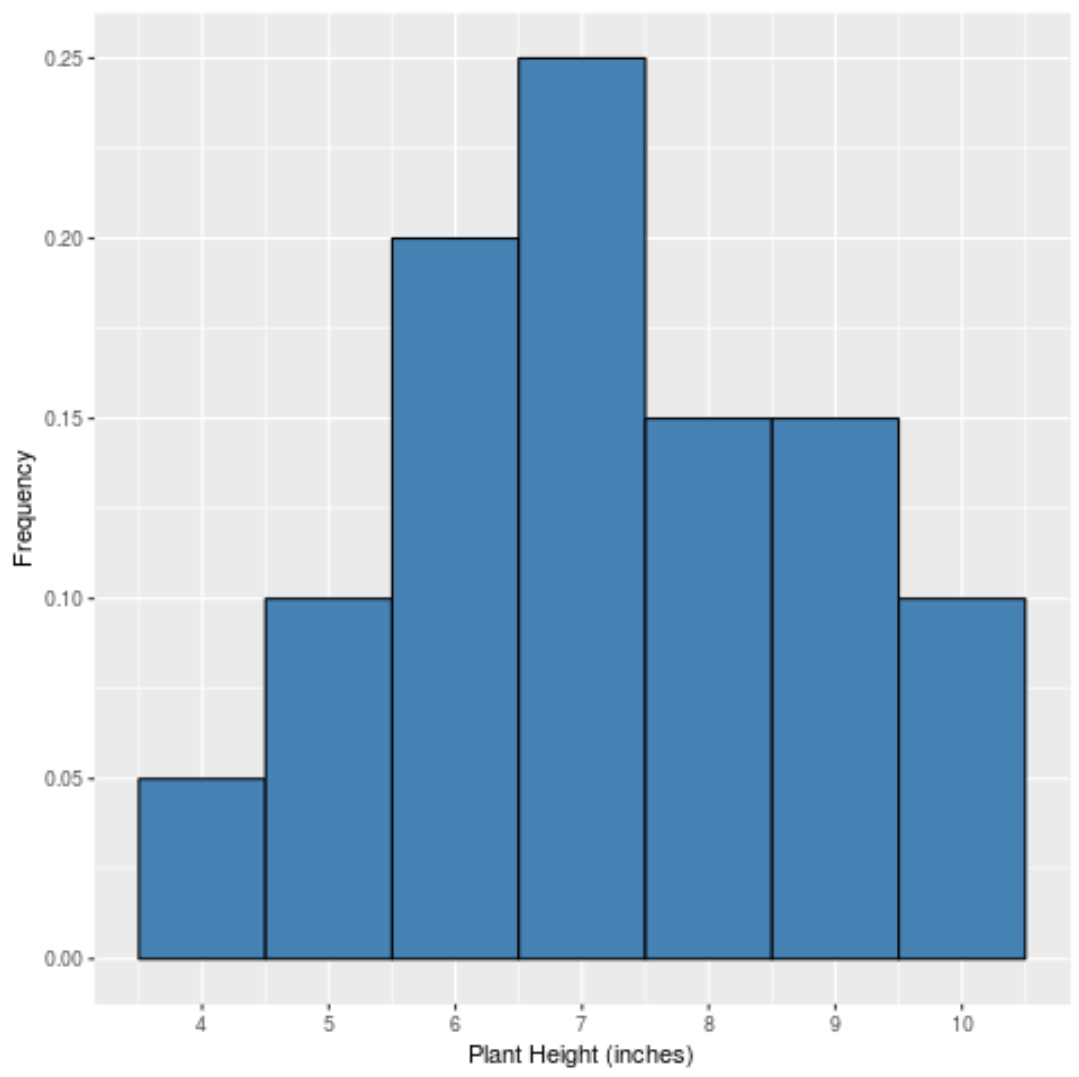
The x-axis shows the data value and the y-axis shows the relative frequency (e.g. the value “7” occurs 5 times out of 20 total values in the dataset, thus it has a relative frequency of 25% or 0.25.
And if we created a density curve to capture the “shape” of this distribution, it would look like this:
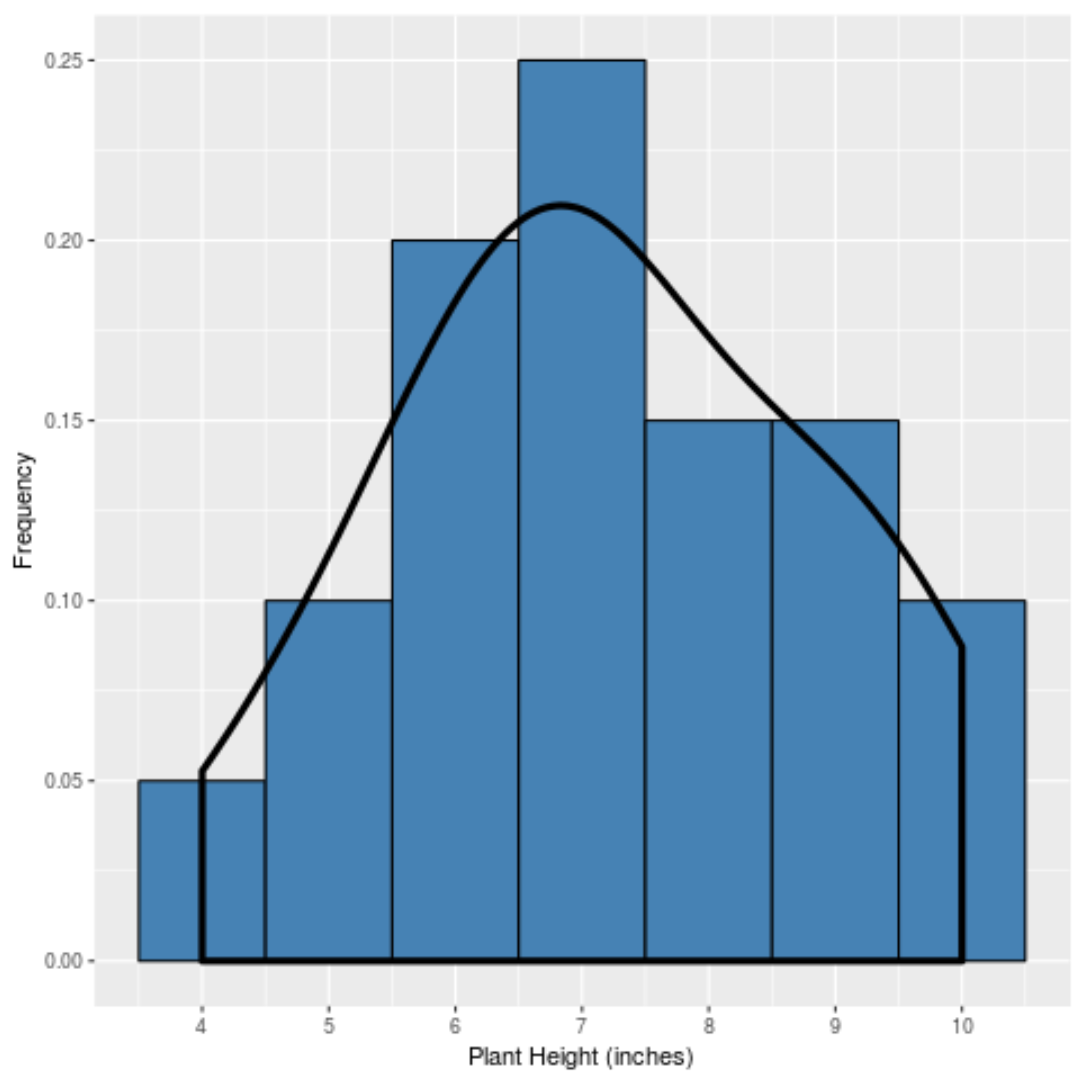
The curve is highest near the center of the distribution because that’s where the most values are located. It’s also lowest near the ends of the distribution because fewer plants take on those values (e.g. a height of 4 inches or 10 inches).
How to Interpret Density Curves
Density curves come in all shapes and sizes and they allow us to gain a quick visual understanding of the distribution of values in a given dataset. In particular, they’re useful for helping us visualize:
1. Skewness
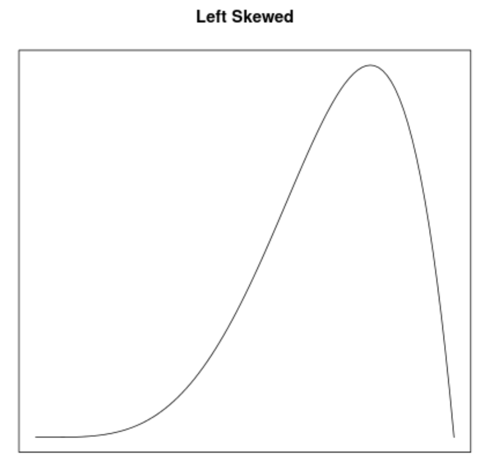
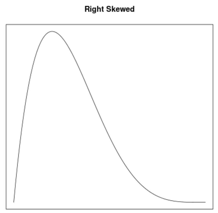
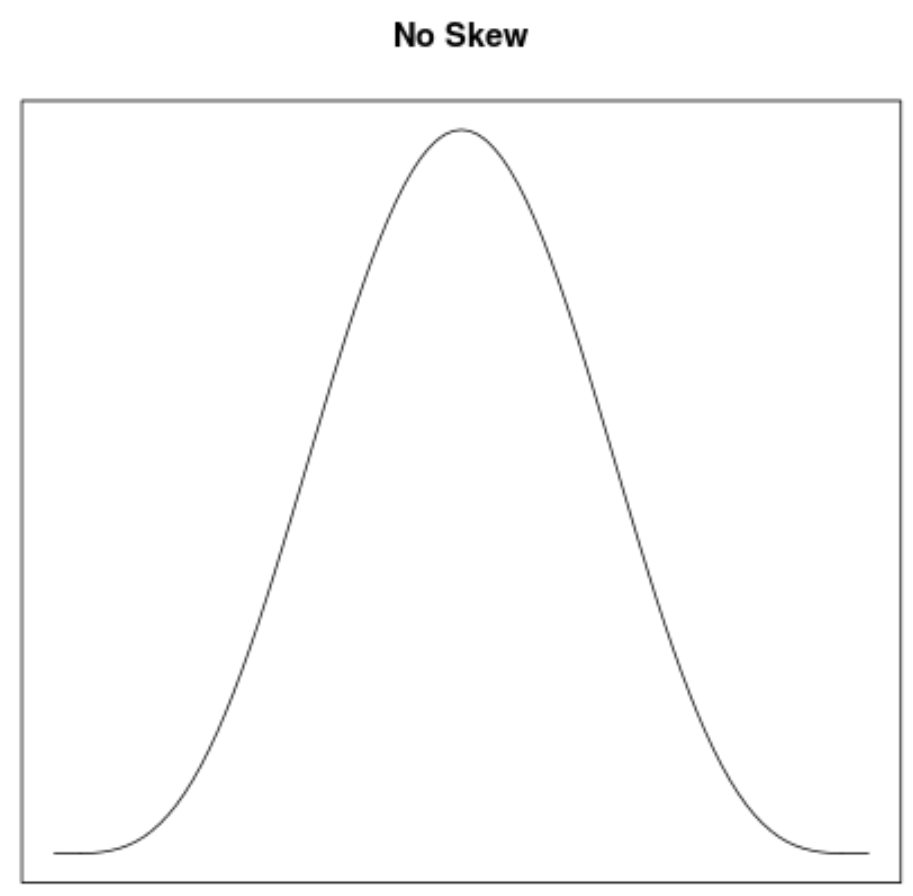
Skewness is a way to describe the symmetry of a distribution. Density curves allow us to quickly see whether or not a graph is left skewed, right skewed, or has no skew:
2. The location of the mean & median
Depending on the skewness of a density curve, we can quickly know whether the mean or median is larger in a given distribution. In particular:
- If a density curve is left skewed, then the mean is less than the median.
- If a density curve is right skewed, then the mean is greater than the median.
- If a density curve has no skew, then the mean is equal to the median.
3. Number of Peaks
Density curves also allow us to quickly see how many “peaks” there are in a given distribution. In each of the examples above, the distributions only had one peak, so we would describe those distributions as unimodal.
However, some distributions can have two peaks which we call bimodal distributions. And in rare cases we can also have multimodal distributions that have two or more peaks.
By simply creating a density curve for a given dataset, we can quickly see how many peaks are in the distribution.
Properties of Density Curves
Density curves have the following properties:
- The area under the curve always adds up to 100%.
- The curve will never dip below the x-axis.
Keep these two facts in mind when you create or interpret density curves for different distributions.
Additional Resources
Introduction to Relative Frequency Histograms
How to Make a Bell Curve in Excel
How to Make a Bell Curve in Python