When we want to compare the means of two independent groups, we can choose between using two different tests:
Student’s t-test: this test assumes that both groups of data are sampled from populations that follow a normal distribution and that both populations have the same variance.
Welch’s t-test: this test assumes that both groups of data are sampled from populations that follow a normal distribution, but it does not assume that those two populations have the same variance.
The Difference Between Student’s t-test and Welch’s t-test
There are two differences in how the Student’s t-test and Welch’s t-test are carried out:
- The test statistic
- The degrees of freedom
Student’s t-test:
Test statistic: (x1 – x2) / sp(√1/n1 + 1/n2)
where x1 and x2 are the sample means, n1 and n2 are the sample sizes for sample 1 and sample 2, respectively, and where sp is calculated as:
sp = √ (n1-1)s12 + (n2-1)s22 / (n1+n2-2)
where s12 and s22 are the sample variances.
Degrees of freedom: n1 + n2 – 2
Welch’s t-test
Test statistic: (x1 – x2) / (√s12/n1 + s22/n2)
Degrees of freedom: (s12/n1 + s22/n2)2 / { [ (s12 / n1)2 / (n1 – 1) ] + [ (s22 / n2)2 / (n2 – 1) ] }
The formula to calculate the degrees of freedom for Welch’s t-test takes into account the difference between the two standard deviations. If the two samples have the same standard deviations, though, then the degrees of freedom for the Welch’s t-test will be the exact same as the degrees of freedom for the Student’s t-test.
Typically, the standard deviations for the two samples are not the same and thus the degrees of freedom for Welch’s t-test tends to be smaller than the degrees of freedom for Student’s t-test.
It’s also important to note that the degrees of freedom for the Welch’s t-test typically is typically not an integer. If you are conducting the test by hand, it’s best practice to round down to the next lowest integer. If you are using a statistical software like R, the software will be able to hand the decimal value for the degrees of freedom.
When Should You Use Welch’s t-test?
Some people argue that the Welch’s t-test should be the default choice for comparing the means of two independent groups since it performs better than the Student’s t-test when sample sizes and variances are unequal between groups, and it gives identical results when sample sizes are variances are equal.
In practice, when you are comparing the means of two groups it’s unlikely that the standard deviations for each group will be identical. This makes it a good idea to just always use Welch’s t-test, so that you don’t have to make any assumptions about equal variances.
Examples of Using Welch’s t-test
Next, we will perform Welch’s t-test on the following two samples to determine if their populations means differ significantly at a significance level of 0.05:
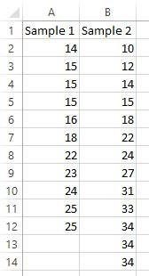
Sample 1: 14, 15, 15, 15, 16, 18, 22, 23, 24, 25, 25
Sample 2: 10, 12, 14, 15, 18, 22, 24, 27, 31, 33, 34, 34, 34
We’ll illustrate how to conduct the test in three different ways:
- By hand
- Using Microsoft Excel
- Using the statistical programming language R
Welch’s t-test by Hand
To conduct Welch’s t-test by hand, we first need to find the sample means, sample variances, and sample sizes:
x1 – 19.27
x2 – 23.69
s12 – 20.42
s22 – 83.23
n1 – 11
n2 – 13
Next, we can plug in these numbers to find the test statistic:
Test statistic: (x1 – x2) / (√s12/n1 + s22/n2)
Test statistic: (19.27 – 23.69) / (√20.42/11 + 83.23/13) = -4.42 / 2.873 = -1.538
Degrees of freedom: (s12/n1 + s22/n2)2 / { [ (s12 / n1)2 / (n1 – 1) ] + [ (s22 / n2)2 / (n2 – 1) ] }
Degrees of freedom: (20.42/11 + 83.23/13)2 / { [ (20.42/11)2 / (11 – 1) ] + [ (83.23/13)2 / (13 – 1) ] } = 18.137. We round this down to the next nearest integer of 18.
Lastly, we will find the t critical value in the t-distribution table that corresponds to a two-tailed test with alpha = .05 for 18 degrees of freedom:
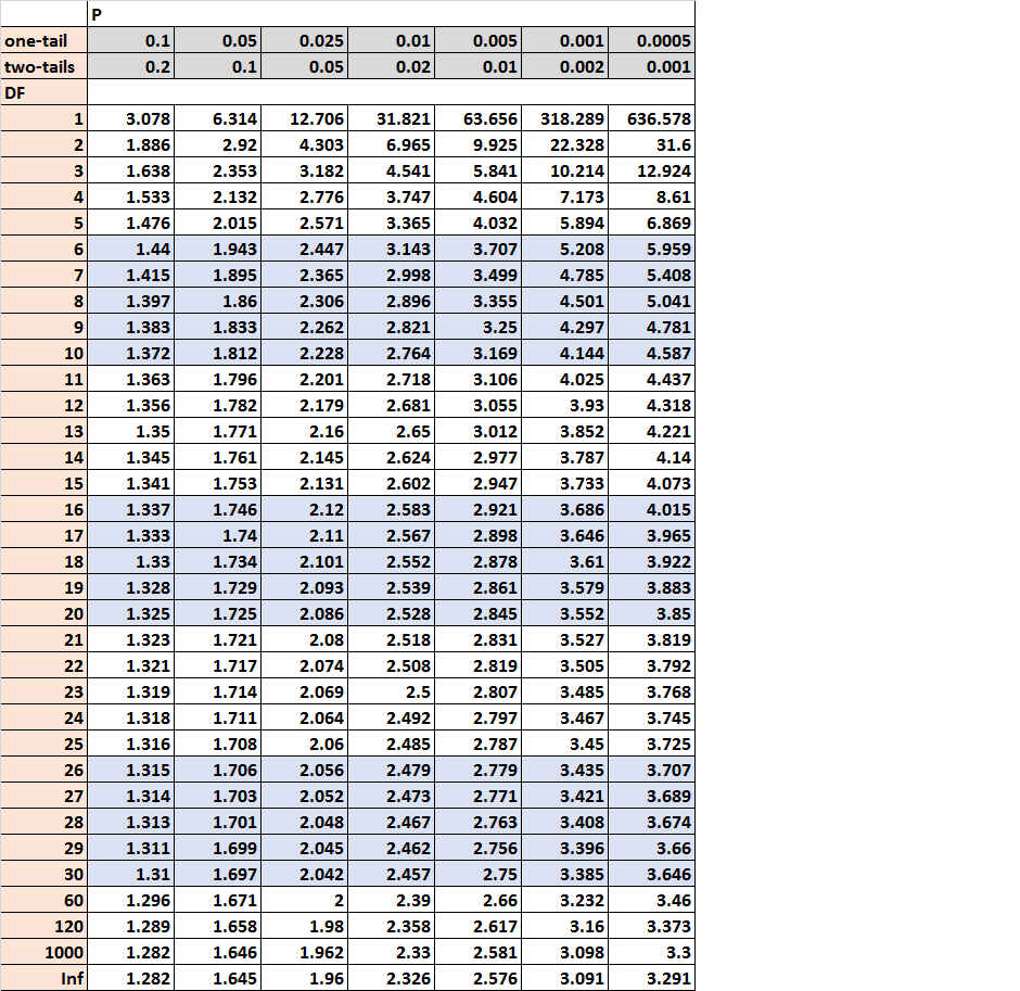
The t critical value is 2.101. Since the absolute value of our test statistic (1.538) is not larger than the t critical value, we fail to reject the null hypothesis of the test. There is not sufficient evidence to say that the means of the two populations are significantly different.
Welch’s t-test Using Excel
To conduct Welch’s t-test in Excel, we first need to download the free Analysis ToolPak. If you don’t already have this downloaded in Excel, I wrote up a quick tutorial on how to download it.
Once you have the Analysis ToolPak downloaded, you can follow the steps below to conduct Welch’s t-test on our two samples:
1. Input the data. Enter the data values for the two samples in columns A and B along with the headers Sample 1 and Sample 2 in the first cell of each column.
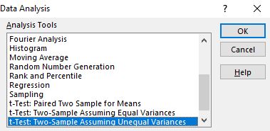
2. Conduct Welch’s t-test using the Analysis ToolPak. Navigate to the Data tab along the top ribbon. Then, under the Analysis group, click the icon for the Analysis ToolPak.

In the box that pops up, click t-Test: Two Sample Assuming Unequal Variances, then click OK.
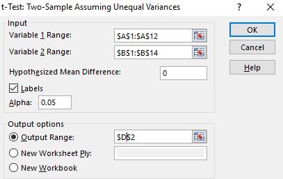
Lastly, fill in the values below and then click OK:
The following output should appear:
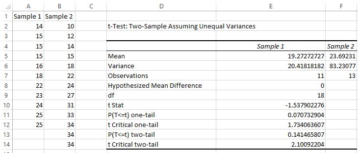
Notice that the results of this test match the results that we got by hand:
- The test statistic is -1.5379.
- The critical two-tail value is 2.1009.
- Since the absolute value of the test statistic is not greater than the critical two-tail value, the two populations means are not statistically different.
- Also, the two-tailed p-value of the test is 0.14, which is larger than 0.05 and confirms that the two population means are not statistically different.
Welch’s t-test Using R
The following code illustrates how to perform Welch’s t-test for our two samples using the statistical programming language R:
#create two vectors to hold sample data values
sample1 #conduct Welch's test
t.test(sample1, sample2)

#	Welch Two Sample t-test
#
#data:  sample1 and sample2
#t = -1.5379, df = 18.137, p-value = 0.1413
#alternative hypothesis: true difference in means is not equal to 0
#95 percent confidence interval:
# -10.453875   1.614714
#sample estimates:
#mean of x mean of y
# 19.27273  23.69231
#
The t.test() function displays the following relevant output:
- t: the test statistic = -1.5379
- df: the degrees of freedom = 18.137
- p-value: the p-value of the two-sided test = 0.1413
- 95% confidence interval: the 95% confidence interval for the true difference in population means = (-10.45, 1.61)
The results of this test match the results we got by hand and by using Excel: the difference in means for these two populations is not statistically significant at the level of alpha = 0.05.