A paired samples t-test is a statistical test that compares the means of two samples when each observation in one sample can be paired with an observation in the other sample.
For example, suppose we want to know whether a certain study program significantly impacts student performance on a particular exam. To test this, we have 20 students in a class take a pre-test. Then, we have each of the students participate in the study program each day for two weeks. Then, the students retake a test of similar difficulty.
To compare the difference between the mean scores on the first and second test, we use a paired t-test because for each student their first test score can be paired with their second test score.
How to Conduct a Paired t-test
To conduct a paired t-test, we can use the following approach:
Step 1: State the null and alternative hypotheses.
H0: μd = 0
Ha: μd ≠ 0 (two-tailed)
Ha: μd > 0 (one-tailed)
Ha: μd (one-tailed)
where μd is the mean difference.
Step 2: Find the test statistic and corresponding p-value.
Let a = the student’s score on the first test and b = the student’s score on the second test. To test the null hypothesis that the true mean difference between the test scores is zero:
- Calculate the difference between each pair of scores (di = bi – ai)
- Calculate the mean difference (d)
- Calculate the standard deviation of the differences sd
- Calculate the t-statistic, which is T = d / (sd / √n)
- Find the corresponding p-value for the t-statistic with n-1 degrees of freedom.
Step 3: Reject or fail to reject the null hypothesis, based on the significance level.
If the p-value is less than our chosen significance level, we reject the null hypothesis and conclude that there is a statistically significant difference between the means of the two groups. Otherwise, we fail to reject the null hypothesis.
How to Conduct a Paired t-test in R
To conduct a paired t-test in R, we can use the built-in t.test() function with the following syntax:
t.test(x, y, paired = TRUE, alternative = “two.sided”)
- x,y: the two numeric vectors we wish to compare
- paired: a logical value specifying that we want to compute a paired t-test
- alternative: the alternative hypothesis. This can be set to “two.sided” (default), “greater” or “less”.
The following example illustrates how to conduct a paired t-test to find out if there is a significant difference in the mean scores between a pre-test and a post-test for 20 students.
Create the Data
First, we’ll create the dataset:
#create the dataset
data #view the dataset
data

#   score group
#1     85   pre
#2     85   pre
#3     78   pre
#4     78   pre
#5     92   pre
#6     94   pre
#7     91   pre
#8     85   pre
#9     72   pre
#10    97   pre
#11    84   pre
#12    95   pre
#13    99   pre
#14    80   pre
#15    90   pre
#16    88   pre
#17    95   pre
#18    90   pre
#19    96   pre
#20    89   pre
#21    84  post
#22    88  post
#23    88  post
#24    90  post
#25    92  post
#26    93  post
#27    91  post
#28    85  post
#29    80  post
#30    93  post
#31    97  post
#32   100  post
#33    93  post
#34    91  post
#35    90  post
#36    87  post
#37    94  post
#38    83  post
#39    92  post
#40    95  post
Visualize the Differences
Next, we’ll look at summary statistics of the two groups using the group_by() and summarise() functions from the dplyr library:
#load dplyr library
library(dplyr)

#find sample size, mean, and standard deviation for each group
data %>%
  group_by(group) %>%
  summarise(
    count = n(),
    mean = mean(score),
    sd = sd(score)
  )

# A tibble: 2 x 4
#  group count  mean    sd
#
#1 post     20  90.3  4.88
#2 pre      20  88.2  7.24
We can also create boxplots using the boxplot() function in R to view the distribution of scores for the pre and post groups:
boxplot(score~group,
  data=data,
  main="Test Scores by Group",
  xlab="Group",
  ylab="Score",
  col="steelblue",
  border="black"
)
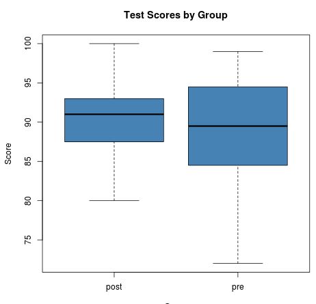
From both the summary statistics and the boxplots, we can see that the mean score in the post group is slightly higher than the mean score in the pre group. We can also see that the scores for the post group have less variability than the scores in the pre group.
To find out if the difference between the means for these two groups is statistically significant, we can proceed to conduct a paired t-test.
Conduct a Paired t-test
Before we conduct the paired t-test, we should check that the distribution of differences is normally (or approximately normally) distributed. To do so, we can create a new vector defined as the difference between the pre and post scores, and perform a shapiro-wilk test for normality on this vector of values:
#define new vector for difference between post and pre scores
differences #perform shapiro-wilk test for normality on this vector of values
shapiro.test(differences)

#	Shapiro-Wilk normality test
#
#data:  differences
#W = 0.92307, p-value = 0.1135
#
The p-value of the test is 0.1135, which is greater than alpha = 0.05. Thus, we fail to reject the null hypothesis that our data is normally distributed. This means we can now proceed to conduct the paired t-test.
We can use the following code to conduct a paired t-test:
t.test(score ~ group, data = data, paired = TRUE)

#	Paired t-test
#
#data:  score by group
#t = 1.588, df = 19, p-value = 0.1288
#alternative hypothesis: true difference in means is not equal to 0
#95 percent confidence interval:
# -0.6837307  4.9837307
#sample estimates:
#mean of the differences
#                   2.15
From the output, we can see that:
- The test statistic t is 1.588.
- The p-value for this test statistic with 19 degrees of freedom (df) is 0.1288.
- The 95% confidence interval for the mean difference is (-0.6837, 4.9837).
- The mean difference between the scores for the pre and post group is 2.15.
Thus, since our p-value is less than our significance level of 0.05 we will fail to reject the null hypothesis that the two groups have statistically significant means.
In other words, we do not have sufficient evidence to say that the mean scores between the pre and post groups are statistically significantly different. This means the study program had no significant effect on test scores.
In addition, our 95% confidence interval says that we are “95% confident” that the true mean difference between the two groups is between -0.6837 and 4.9837.
Since the value zero is contained in this confidence interval, this means that zero could in fact be the true difference between the mean scores, which is why we failed to reject the null hypothesis in this case.