The easiest way to count the number of cells in a filtered range in Excel is to use the following syntax:
SUBTOTAL(103, A1:A10)
Note that the value 103 is a shortcut for finding the count of a filtered range of rows.
The following example shows how to use this function in practice.
Example: Count Filtered Rows in Excel
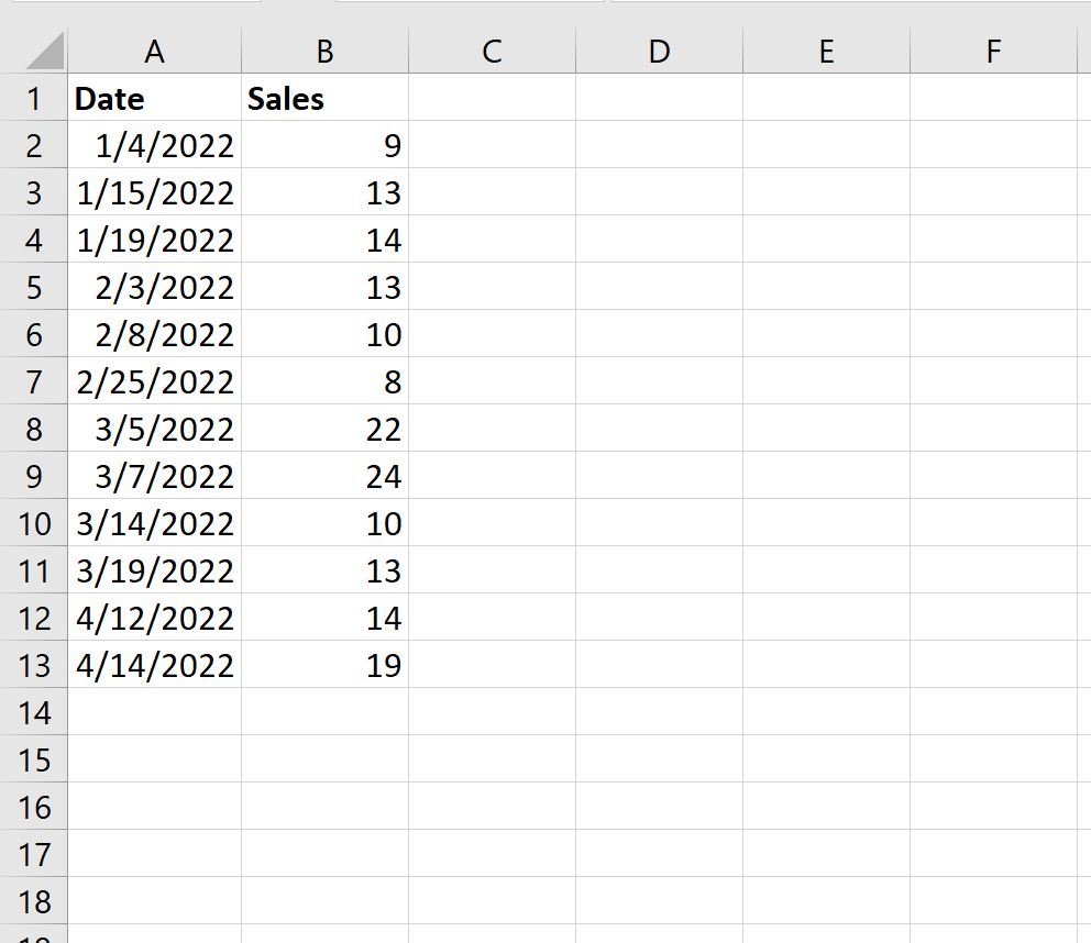
Suppose we have the following dataset that shows the number of sales made during various days by a company:
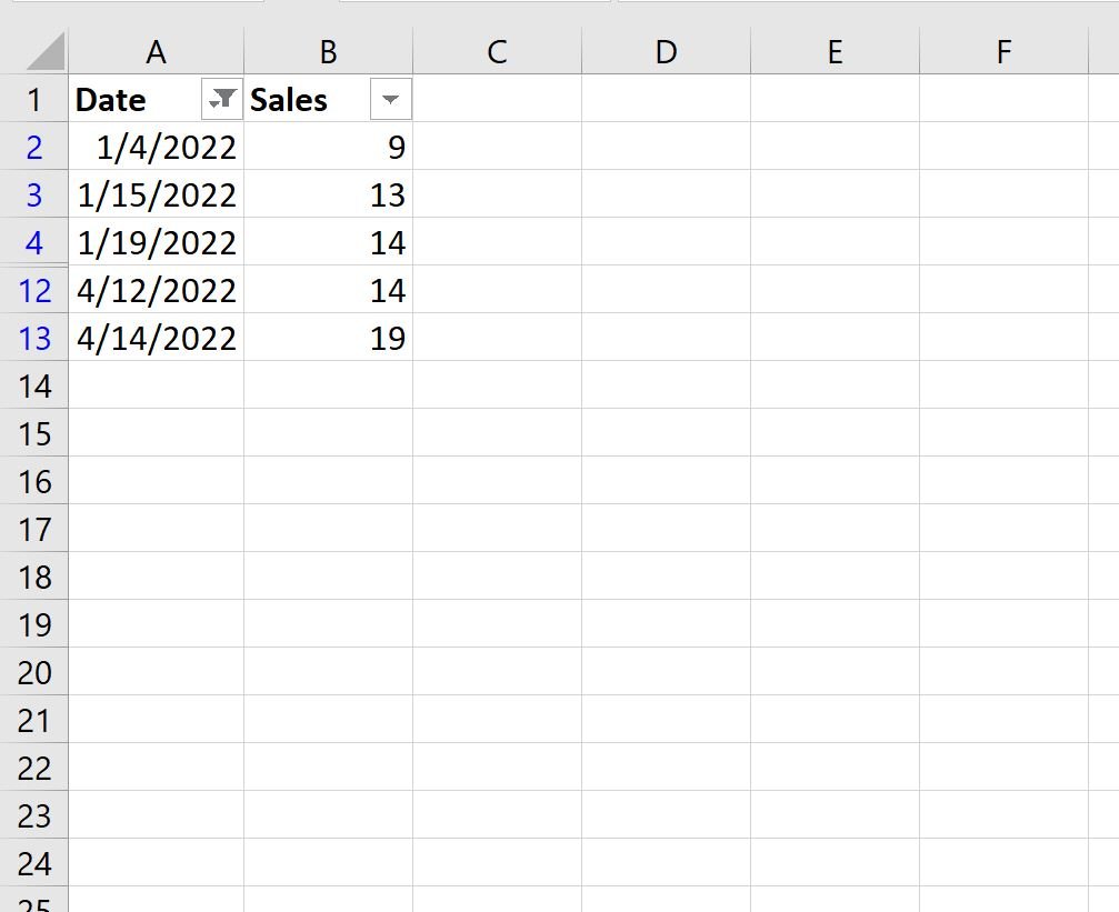
Next, let’s filter the data to only show the dates that are in January or April.
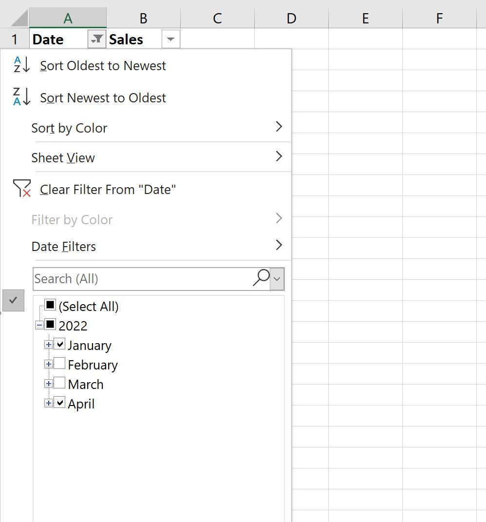
To do so, highlight the cell range A1:B13. Then click the Data tab along the top ribbon and click the Filter button.

Then click the dropdown arrow next to Date and make sure that only the boxes next to January and April are checked, then click OK:
The data will automatically be filtered to only show the rows where the dates are in January or April:
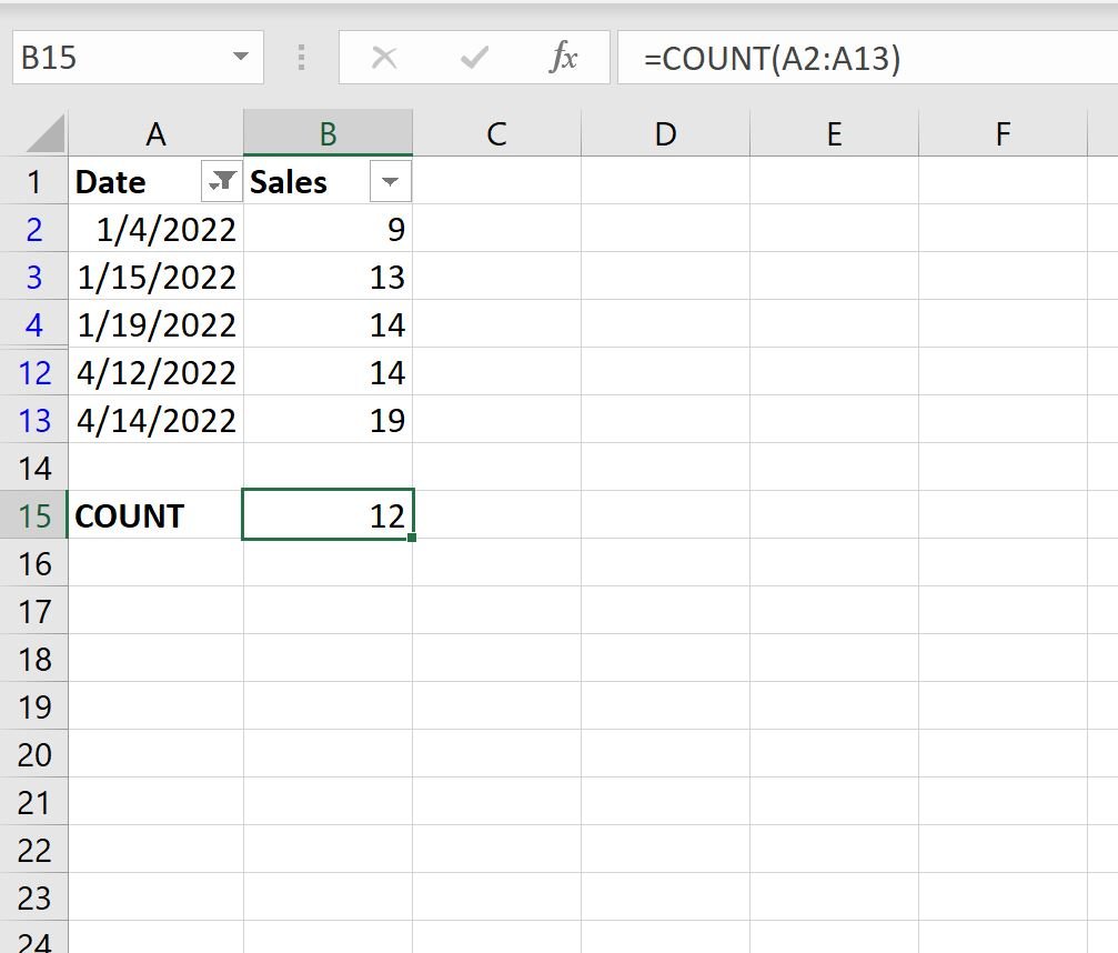
If we attempt to use the COUNT() function to count the number of values in the Date column, it will actually return the count of all of the original values:
Instead, we can use the SUBTOTAL() function:
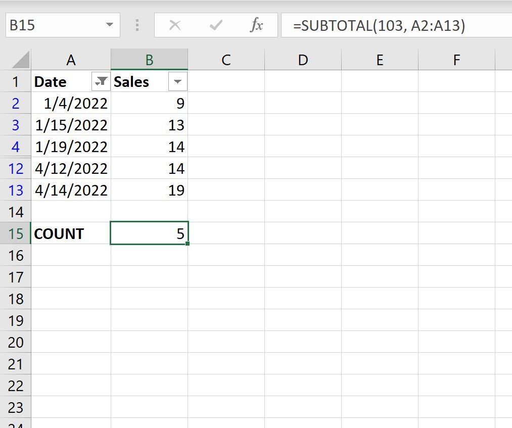
This function only counts the visible rows.
From the output we can see that there are 5 days that fall in January or April.
Note that in this particular formula we used 103 in the subtotal function, but we could have also used 102:
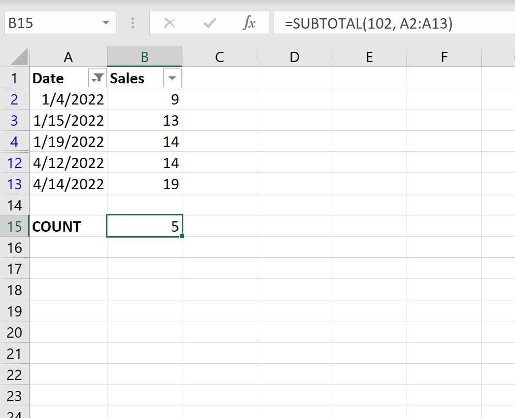
Here’s the difference between the two:
- 102 uses the COUNT function, which counts only cells containing numbers.
- 103 uses the COUNTA function, which counts all cells that aren’t empty.
Feel free to use the value in your formula that makes sense for your data.
Additional Resources
The following tutorials explain how to perform other common operations in Excel:
How to Delete Filtered Rows in Excel
How to Sum Filtered Rows in Excel
How to Average Filtered Rows in Excel