Often you may want to apply conditional formatting to cells based on multiple conditions in Excel.
The following example shows exactly how to do so.
Example: Conditional Formatting with Multiple Conditions
Suppose we have the following dataset that contains information about various basketball teams:

Suppose we would like to highlight each value in the points column where the value is greater than 10 and less than 20.
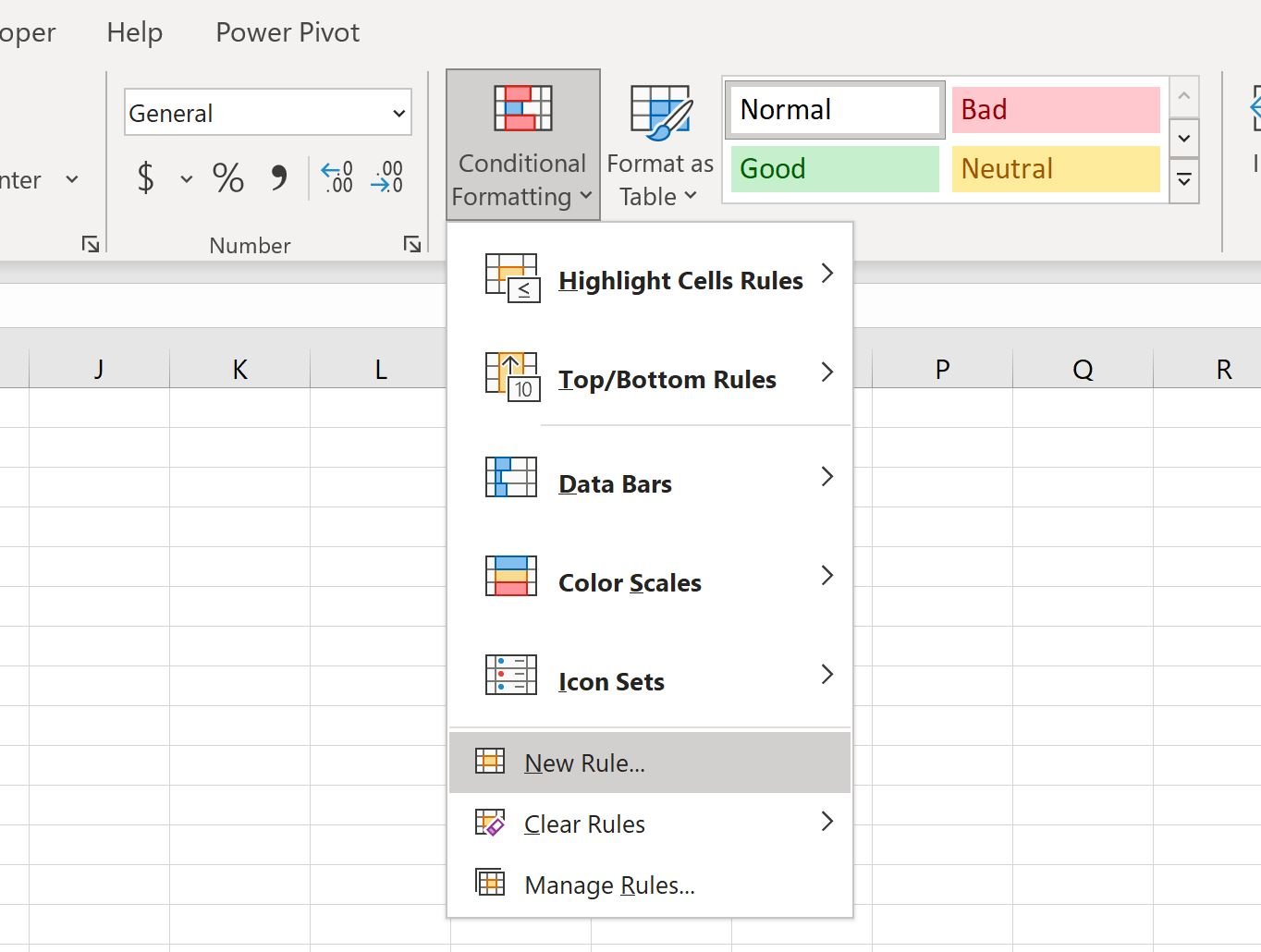
To do so, highlight the values in the range B2:B14, then click the Conditional Formatting icon on the Home tab, then click New Rule:

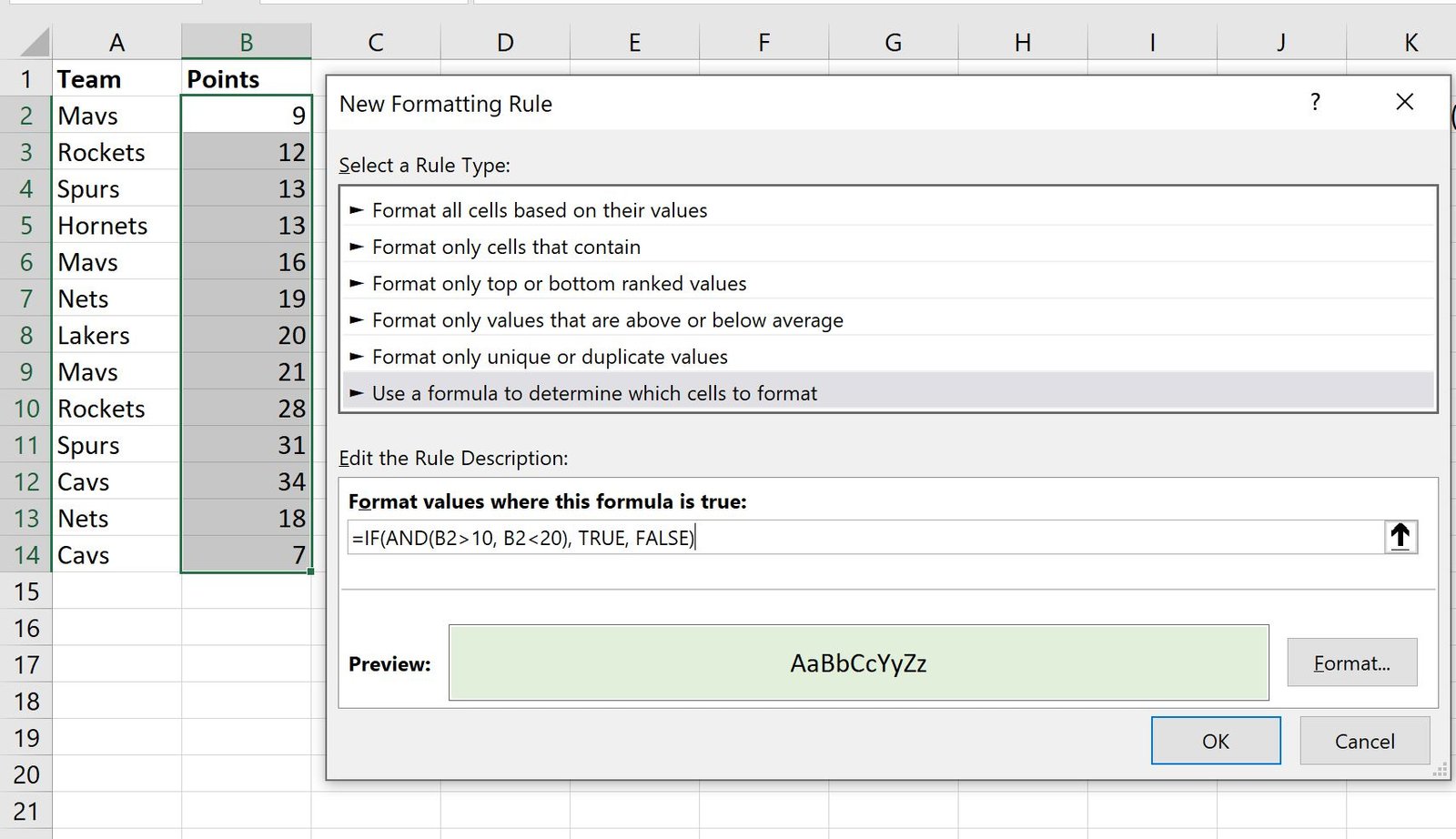
In the new window that appears, click Use a formula to determine which cells to format, then type in the following formula into the box:
=IF(AND(B2>10, B2
Then click the Format button and choose a fill color to use, then click OK:

Each value in the points column that is greater than 10 and less than 20 will automatically be highlighted:

Note: You can find the complete documentation for the AND function in Excel here.
Additional Resources
The following tutorials explain how to perform other common tasks in Excel:
How to Apply Conditional Formatting if Cell Contains Text in Excel
How to Find the Top 10% of Values in an Excel Column
How to Find the Top 10 Values in a List in Excel
How to Find Unique Values from Multiple Columns in Excel