How to Perform a Two Sample t-test in SPSS

---

A two sample t-test is used to test whether or not the means of two populations are equal.

This tutorial explains how to conduct a two sample t-test in SPSS.

Example: Two Sample t-test in SPSS

Researchers want to know if a new fuel treatment leads to a change in the average miles per gallon of a certain car. To test this, they conduct an experiment in which 12 cars receive the new fuel treatment and 12 cars do not.

The following screenshot shows the mpg for each car along with the group they belong to (0 = no fuel treatment, 1 = fuel treatment):

Use the following steps to perform a two sample t-test to determine if there is a difference in average mpg between these two groups, based on the following null and alternative hypotheses:

• H₀: μ₁ = μ₂ (average mpg between the two populations is equal)
• H₁: μ₁ ≠ μ₂ (average mpg between the two populations is not equal)

Use a significance level of α = 0.05.

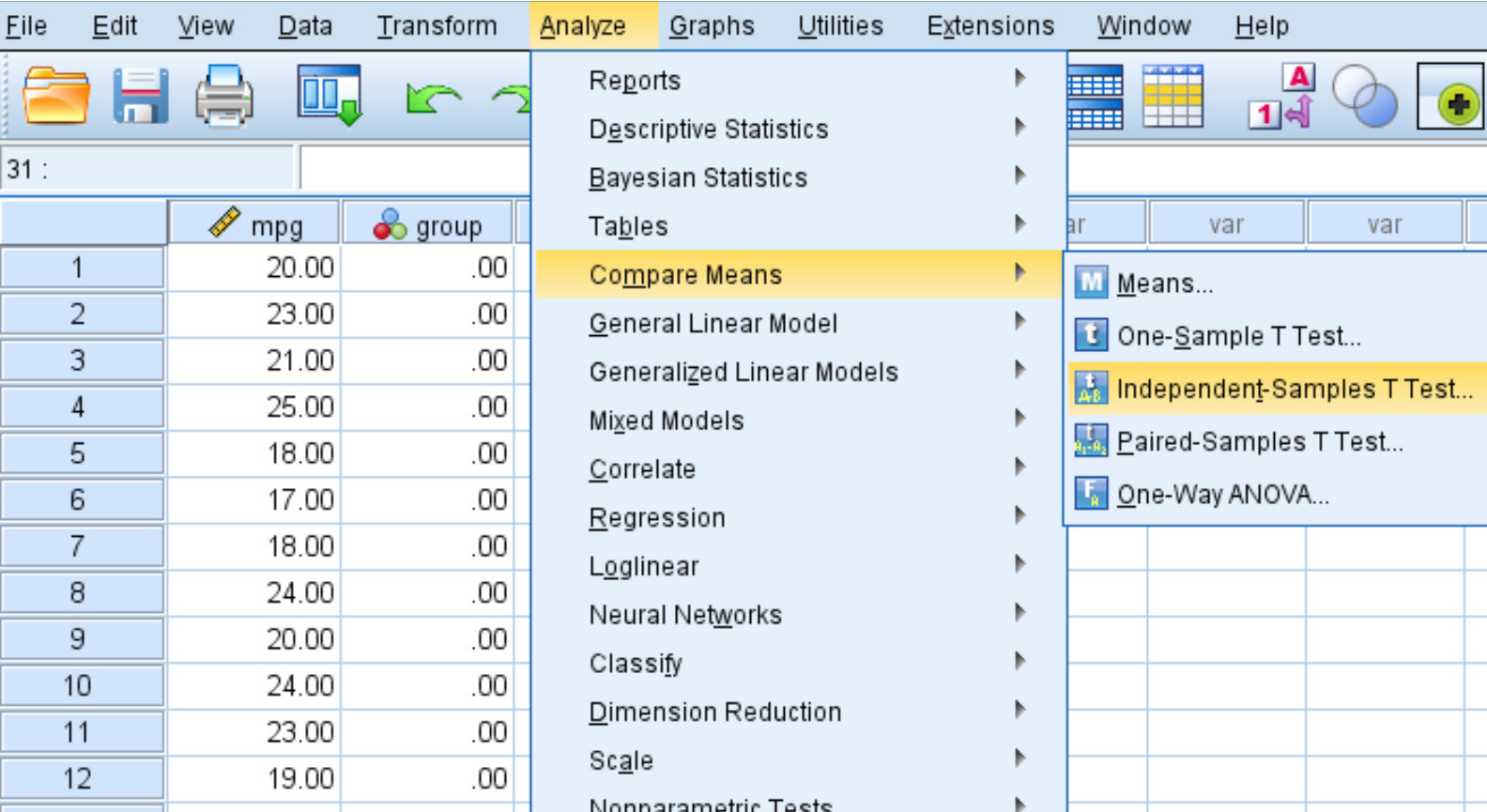
Step 1: Choose the Independent Samples T Test option.

Click the Analyze tab, then Compare Means, then Independent-Samples T Test:

Step 2: Fill in the necessary values to perform the two sample t-test.

Once you click Independent-Samples T Test, the following window will appear:

Drag the mpg into the box labelled Test Variable(s) and group into the box labelled Grouping Variable. Then click Define Groups and define Group 1 as the rows with value 0 and define Group 2 as the rows with value 1. Then click OK.

Step 3: Interpret the results.

Once you click OK, the results of the two sample t-test will be displayed:

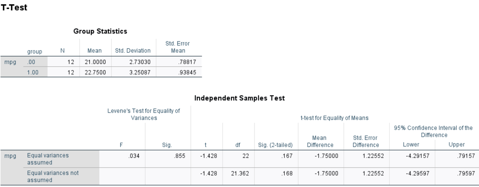
The first table displays the following summary statistics for both groups:

• N: The sample size
• Mean: The mean mpg of cars in each group
• Std. Deviation: The standard deviation of the mpg of cars in each group
• Std. Error Mean: The standard error of the mean mpg, calculated as s/√n

The second table displays the results of the two sample t-test. The first row shows the results of the test if you assume that the variance between the two groups is equal. The second row shows the results of the test if you don’t make this assumption. 

In this case, the two versions of the test produce nearly identical results. Thus, we will simply refer to the results of the first row:

• t: The test statistic, found to be -1.428
• df: The degrees of freedom, calculated as n₁+n₂-2 = 12+12-2 = 22
• Sig. (2-tailed): The two-sided p-value that corresponds to a t value of -1.428 with df=22
• Mean Difference: The difference between the two sample means
• Std. Error Difference: The standard error of the mean difference
• 95% C.I. of the Difference: The 95% confidence interval for the true difference between the two population means

Since the p-value of the test (.167) is not less than 0.05, we fail to reject the null hypothesis. We do not have sufficient evidence to say that the true mean mpg is different between cars that receive treatment and cars that don’t.