How to Create a t-Distribution Graph in Excel

A t-distribution is a type of continuous probability distribution. It has the following properties:

It is continuous
It is bell-shaped
It is symmetric around zero
It is defined by one parameter: the number of degrees of freedom
The t-distribution converges to the standard normal distribution as the number of degrees of freedom converges to infinity

The t-distribution is often used in various hypothesis tests when sample sizes are small (n the normal distribution.

Often we are interested in visualizing the t-distribution. Fortunately, it’s easy to create a t-distribution graph in Excel by using the T.DIST() function which uses the following syntax:

T.DIST(x, deg_freedom, cumulative)

x: the value for the random variable in the t-distribution
deg_freedom: an integer that indicates the number of degrees of freedom in the t-distribution
cumulative: when set to TRUE, it returns the value for the cumulative density function; when set to FALSE, it returns the value for the probability density function

Next, we’ll show how to create the following t-distribution graph in Excel:

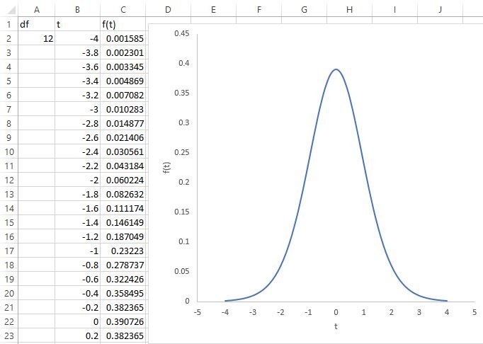
To create a t-distribution graph in Excel, we can perform the following steps:

1. Enter the number of degrees of freedom (df) in cell A2. In this case, we will use 12.

2. Create a column for the range of values for the random variable in the t-distribution. In this case, we will create a range of values from -4 to 4 by increments of 2 in cells B2 through B42.

3. Create a column for the pdf of the t-distribution associated with the random values. In cell C2, type the formula T.DIST(B2, $A$2, FALSE). Then hover over the bottom right of cell C2 until the + sign appears. Click and drag down to autofill the values for cells C2 through C42.

4. Create the graph. Highlight the two columns (B2:C42). Click the INSERT tab. In the Charts area, click scatter with smooth lines. The following chart will appear:

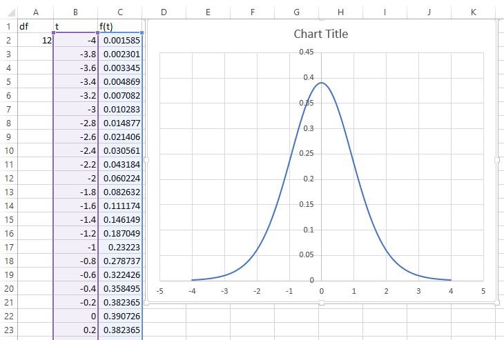
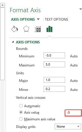
5. Change the graph appearance. By default, the y-axis appears in the middle of the graph and the gridlines show up in the background. We can change this by using the following steps:

Right click on the x-axis. Click Format Axis. Under Vertical axis crosses, click Axis Value and type in -5.

Click inside the chart. A + sign will appear in the top right corner. Click it to remove the gridlines (if you’d like) and add axes titles. In this example, we choose to label the x-axis as t, labelthe y-axis as f(t), and remove the title entirely. The picture below shows the end result:

How to Create Several t-Distribution Graphs in Excel

We can also display several t-distribution curves in one graph if we’d like. This can be useful if we want to see how the shape of the t-distribution changes for various values for the degrees of freedom.

In order to display several t-distribution curves, we simply need to add three new columns for a t-distribution with a different value for the degrees of freedom. For example, we can create t-distribution curves for degrees of freedom = 6 and degrees of freedom = 60:

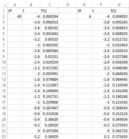
To create the t-distribution curve for df = 60, we can use the exact same steps we used before. To add a curve for df = 6, we can perform the following steps:

Right click inside the chart. Click Select Data.
Under Legend Entries (Series), click Edit.
Choose the cells for the X Values and Y Values that contain the values in columns F and G. Then click OK. The following curve will be added to the chart:

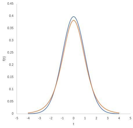
You’ll notice a pattern for t-distribution graphs:

The higher the degrees of freedom, the more narrow the t-distribution curve will be. That is, it will have a higher peak.
Conversely, the lower the degrees of freedom, the more flattened out the curve will be and the “fatter” the tails of the graph will be.
As the degrees of freedom approaches infinity, the curve will converge to the standard normal distribution curve.

Modifying the Aesthetics of the Graph

Note that you can also modify the aesthetics of the graph by changing the following features:

Modify the size and color of the title
Modify the size and color of the axes labels
Choose whether or not to display gridlines in the background
Modify the background color of the graph
Modify the color of the curve itself
Choose whether or not to display the tick marks along the axes

Depending on how you would like the graph to appear, Excel gives you the ability to modify the chart quite a bit.

Find more Excel tutorials on Statology here.