Pivot tables offer an easy way to summarize the values of a dataset.

This tutorial provides a step-by-step example of how to create and format a pivot table for a raw dataset in Google Sheets.
Step 1: Enter the Data
First, let’s enter some sales data for an imaginary company:

Step 2: Create the Pivot Table
Next, highlight all of the data. Along the top ribbon, click Data and then click Pivot table.

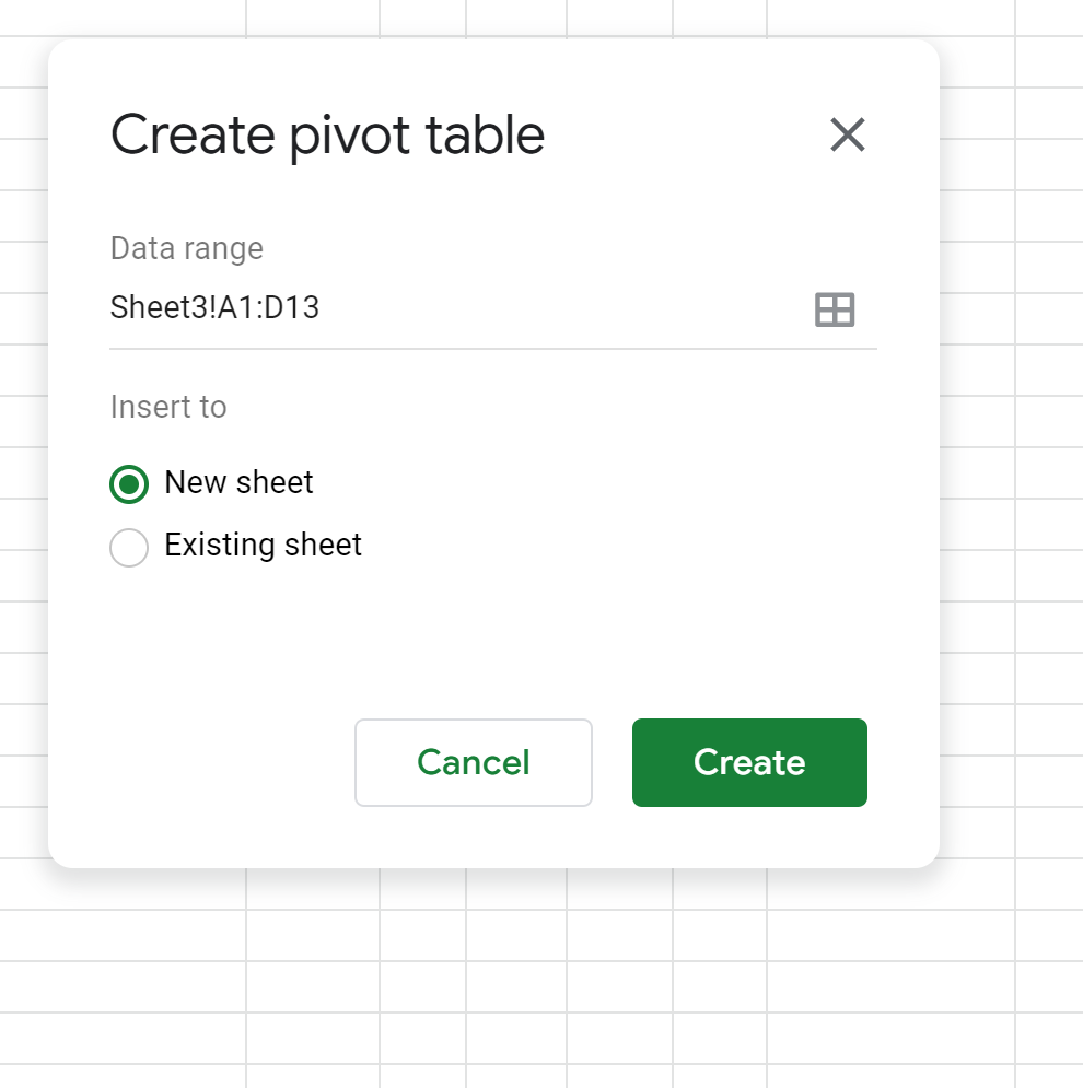
Choose to enter the pivot table in a new sheet or an existing sheet, then click Create.
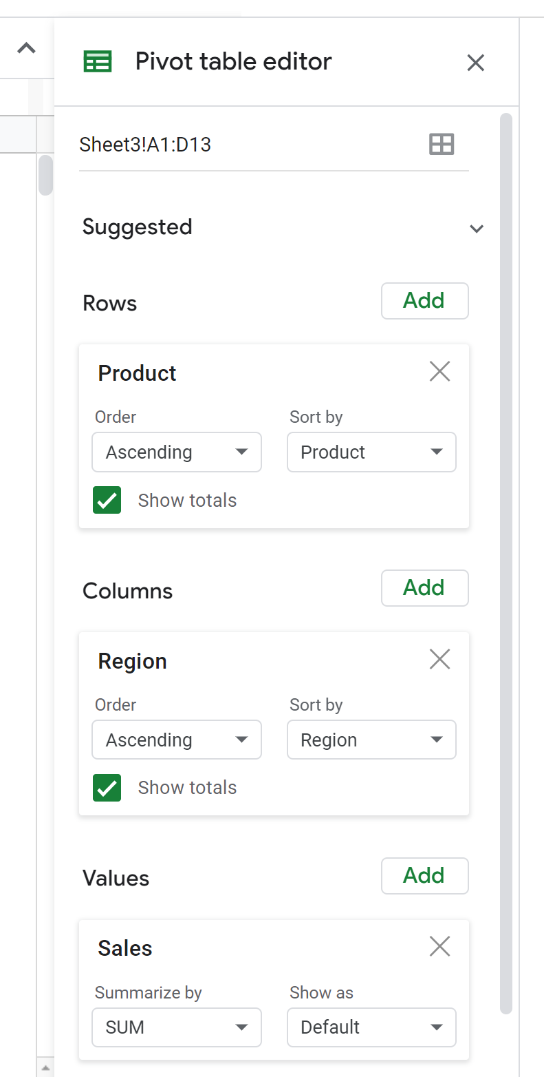
In the pivot table editor that appears to the right, add the Product to the Rows, Region to the Columns, and Sales to the Values.
Our pivot table will now look like this:

Step 3: Choose a Custom Theme
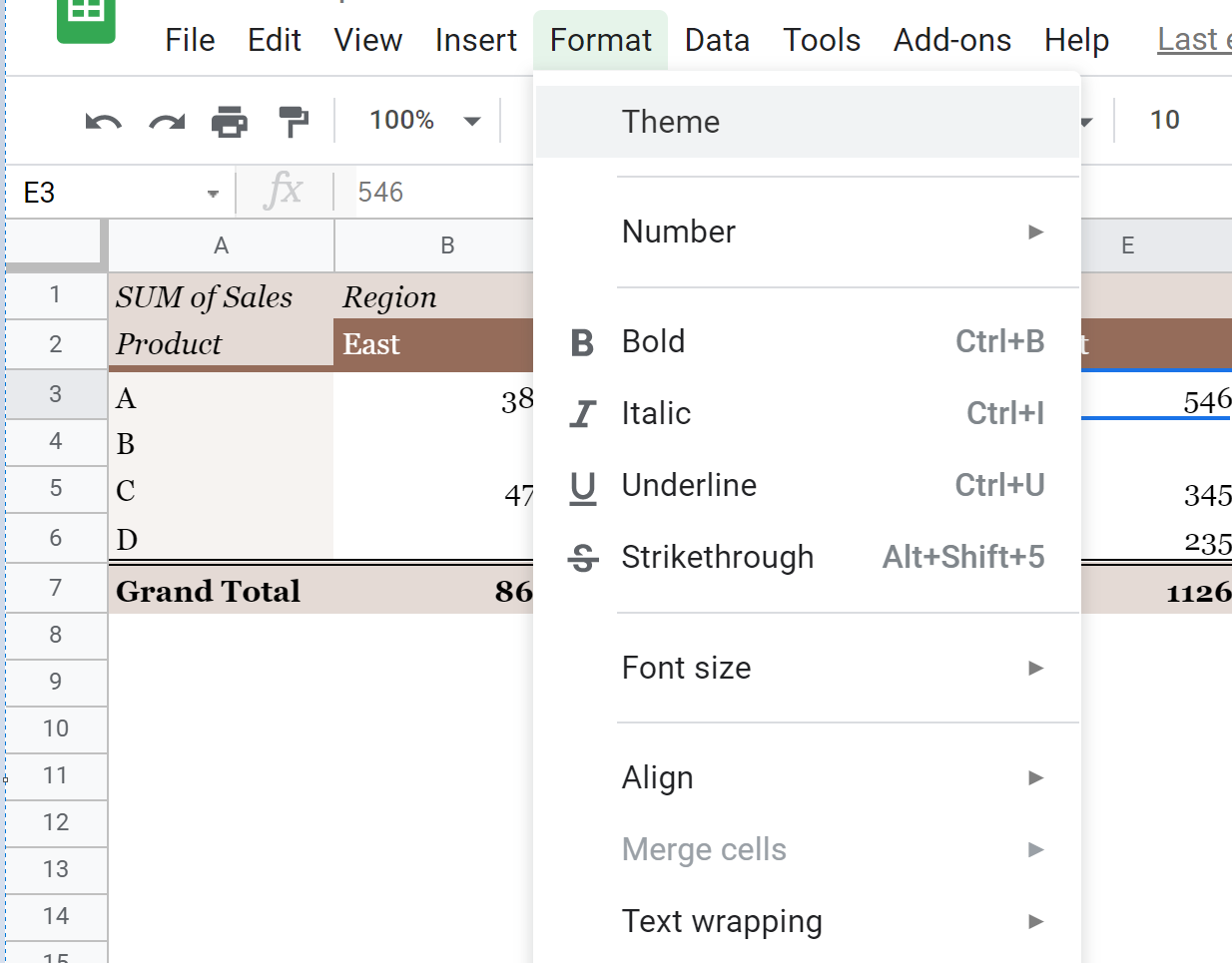
Next, click the Format tab along the top ribbon and click Theme:
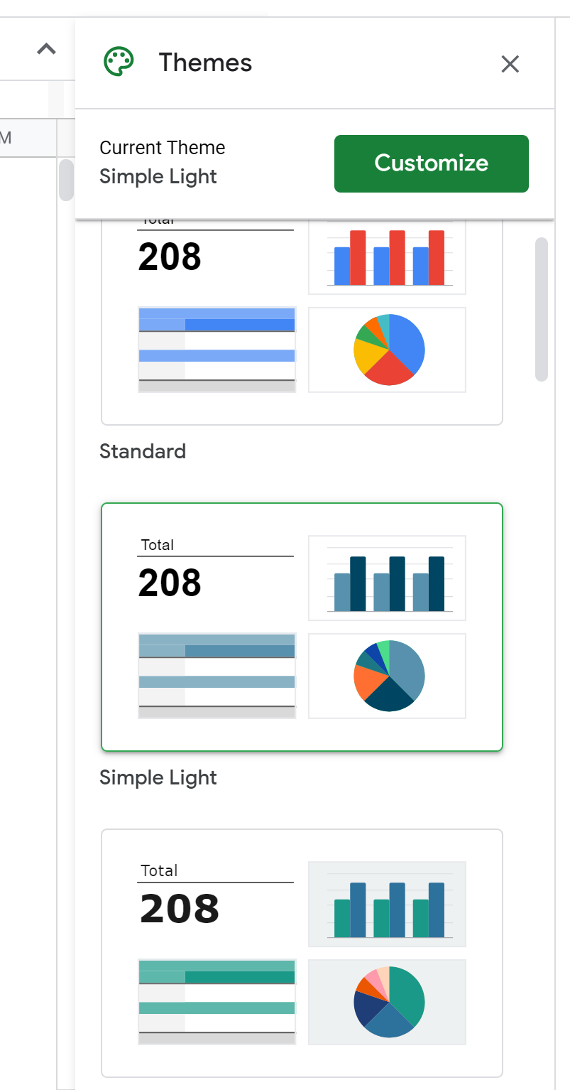
In the window that appears to the right, click any theme you’d like for the pivot table. Or you can click Customize to choose your own theme colors.
We’ll choose the Simple Light theme:
Step 4: Add a Border & Center the Text
Next, we’ll highlight all of the data and add a border around each cell:
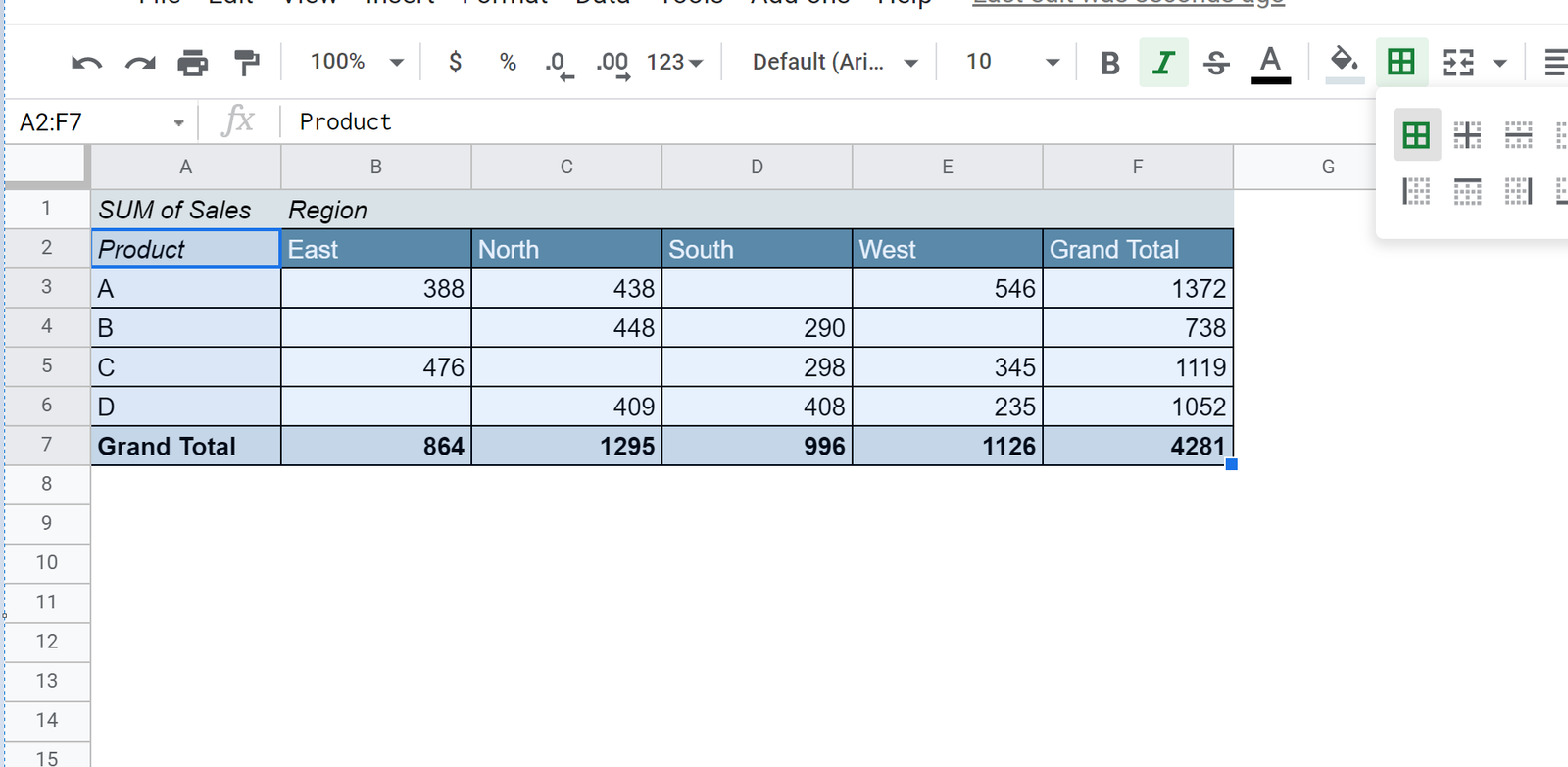
Lastly, we’ll center the data values inside the pivot table:
The pivot table is now formatted to look neat and clean.
You can find more Google Sheets tutorials on this page.