Developed by biostatistician Karl Pearson, Pearson’s coefficient of skewness is a way to measure the skewness in a sample dataset.
There are actually two methods that can be used to calculate Pearson’s coefficient of skewness:
Method 1: Using the Mode
Skewness = (Mean – Mode) / Sample standard deviation
Method 2: Using the Median
Skewness = 3(Mean – Median) / Sample standard deviation
In general, the second method is preferred because the mode is not always a good indication of where the “central” value of a dataset lies and there can be more than one mode in a given dataset.
The following step-by-step example shows how to calculate both versions of the Pearson’s coefficient of skewness for a given dataset in Excel.
Step 1: Create the Dataset
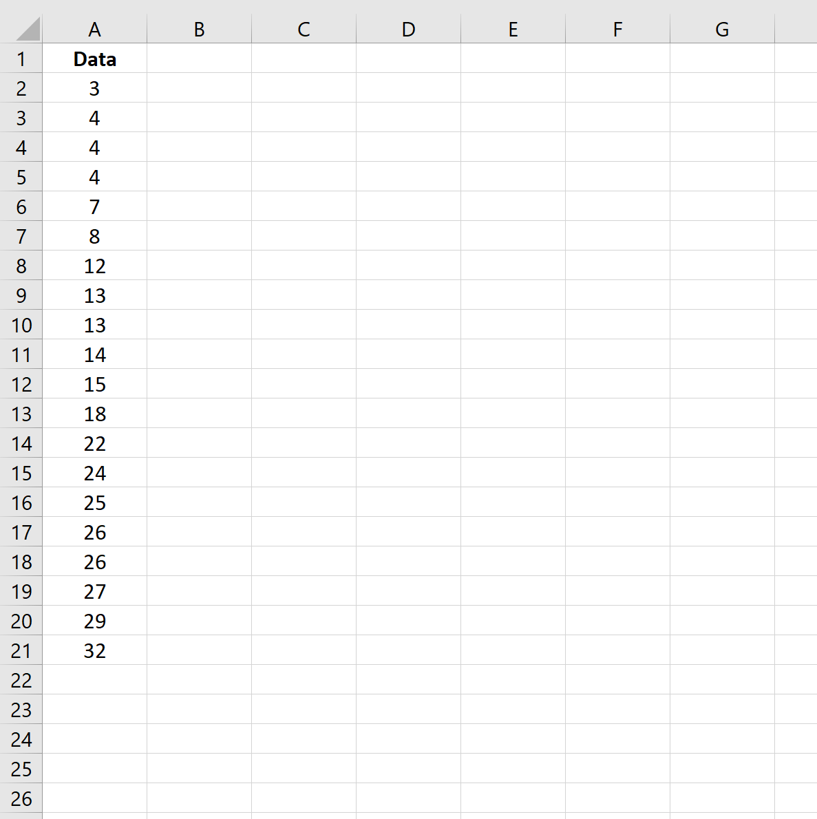
First, let’s create the following dataset in Excel:

Step 2: Calculate the Pearson Coefficient of Skewness (Using the Mode)
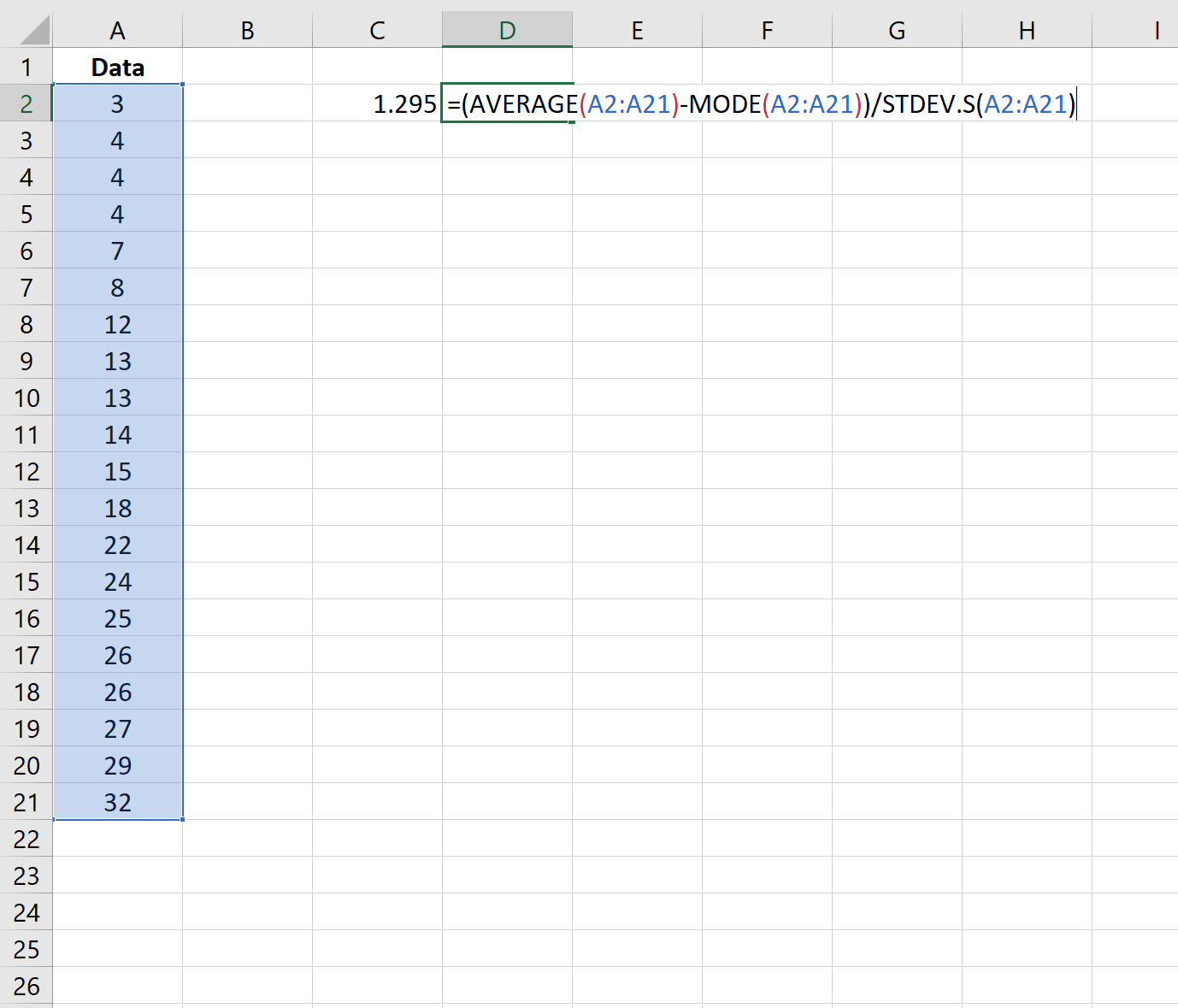
Next, we can use the following formula to calculate the Pearson Coefficient of Skewness using the mode:

The skewness turns out to be 1.295.
Step 3: Calculate the Pearson Coefficient of Skewness (Using the Median)
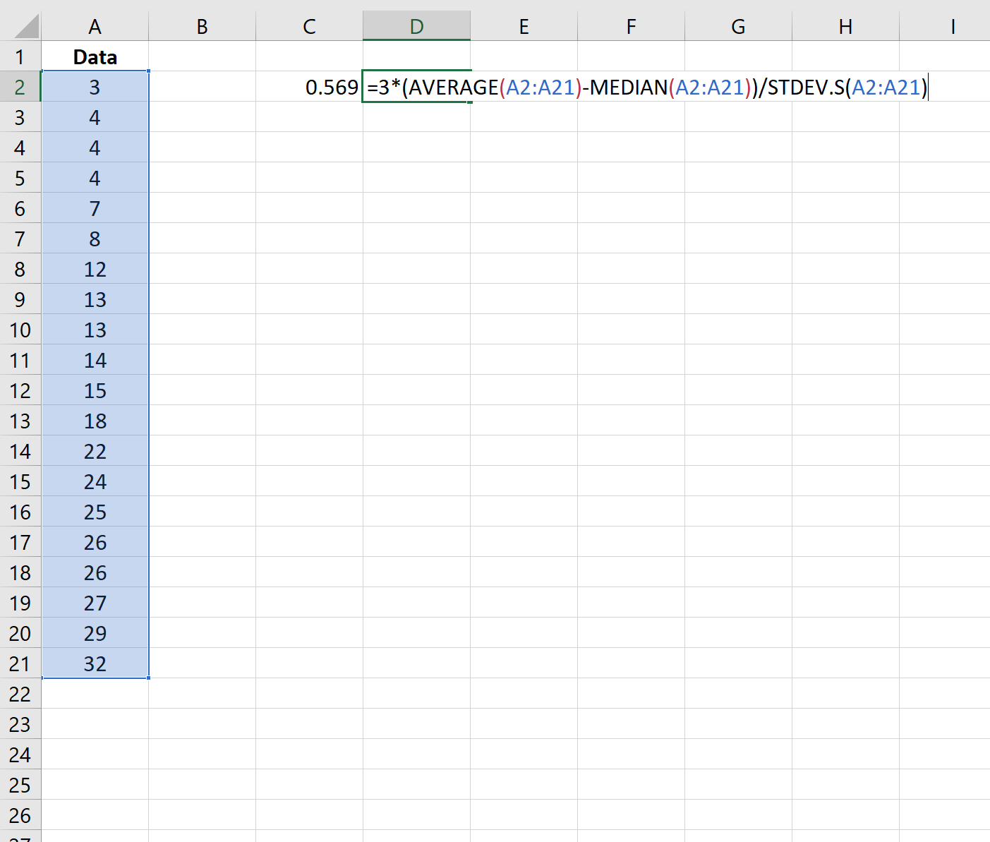
We can also use the following formula to calculate the Pearson Coefficient of Skewness using the median:

The skewness turns out to be 0.569.
How to Interpret Skewness
We interpret the Pearson coefficient of skewness in the following ways:
- A value of 0 indicates no skewness. If we created a histogram to visualize the distribution of values in a dataset, it would be perfectly symmetrical.
- A positive value indicates positive skew or “right” skew. A histogram would reveal a “tail” on the right side of the distribution.
- A negative value indicates a negative skew or “left” skew. A histogram would reveal a “tail” on the left side of the distribution.
In our previous example, the skewness was positive which indicates that the distribution of data values was positively skewed or “right” skewed.
Additional Resources
Check out this article for a nice explanation of left skewed vs. right skewed distributions.