Many statistical tests make the assumption that the residuals of a response variable are normally distributed.
However, often the residuals are not normally distributed. One way to address this issue is to transform the response variable using one of the three transformations:
1. Log Transformation: Transform the response variable from y to log(y).
2. Square Root Transformation: Transform the response variable from y to √y.
3. Cube Root Transformation: Transform the response variable from y to y1/3.
By performing these transformations, the response variable typically becomes closer to normally distributed. The following examples show how to perform these transformations in R.
Log Transformation in R
The following code shows how to perform a log transformation on a response variable:
#create data frame
df #perform log transformation
log_y
The following code shows how to create histograms to view the distribution of y before and after performing a log transformation:
#create histogram for original distribution
hist(df$y, col='steelblue', main='Original')

#create histogram for log-transformed distribution
hist(log_y, col='coral2', main='Log Transformed')
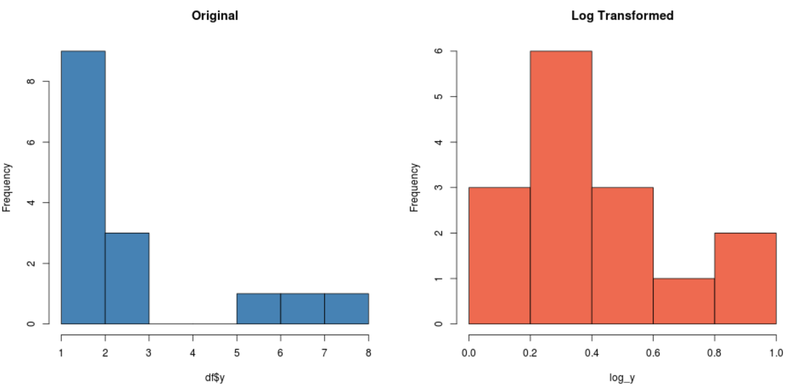
Notice how the log-transformed distribution is much more normal compared to the original distribution. It’s still not a perfect “bell shape” but it’s closer to a normal distribution that the original distribution.
In fact, if we perform a Shapiro-Wilk test on each distribution we’ll find that the original distribution fails the normality assumption while the log-transformed distribution does not (at α = .05):
#perform Shapiro-Wilk Test on original data
shapiro.test(df$y)

	Shapiro-Wilk normality test

data:  df$y
W = 0.77225, p-value = 0.001655

#perform Shapiro-Wilk Test on log-transformed data
shapiro.test(log_y)

	Shapiro-Wilk normality test

data:  log_y
W = 0.89089, p-value = 0.06917
Square Root Transformation in R
The following code shows how to perform a square root transformation on a response variable:
#create data frame
df #perform square root transformation
sqrt_y
The following code shows how to create histograms to view the distribution of y before and after performing a square root transformation:
#create histogram for original distribution
hist(df$y, col='steelblue', main='Original')

#create histogram for square root-transformed distribution
hist(sqrt_y, col='coral2', main='Square Root Transformed')
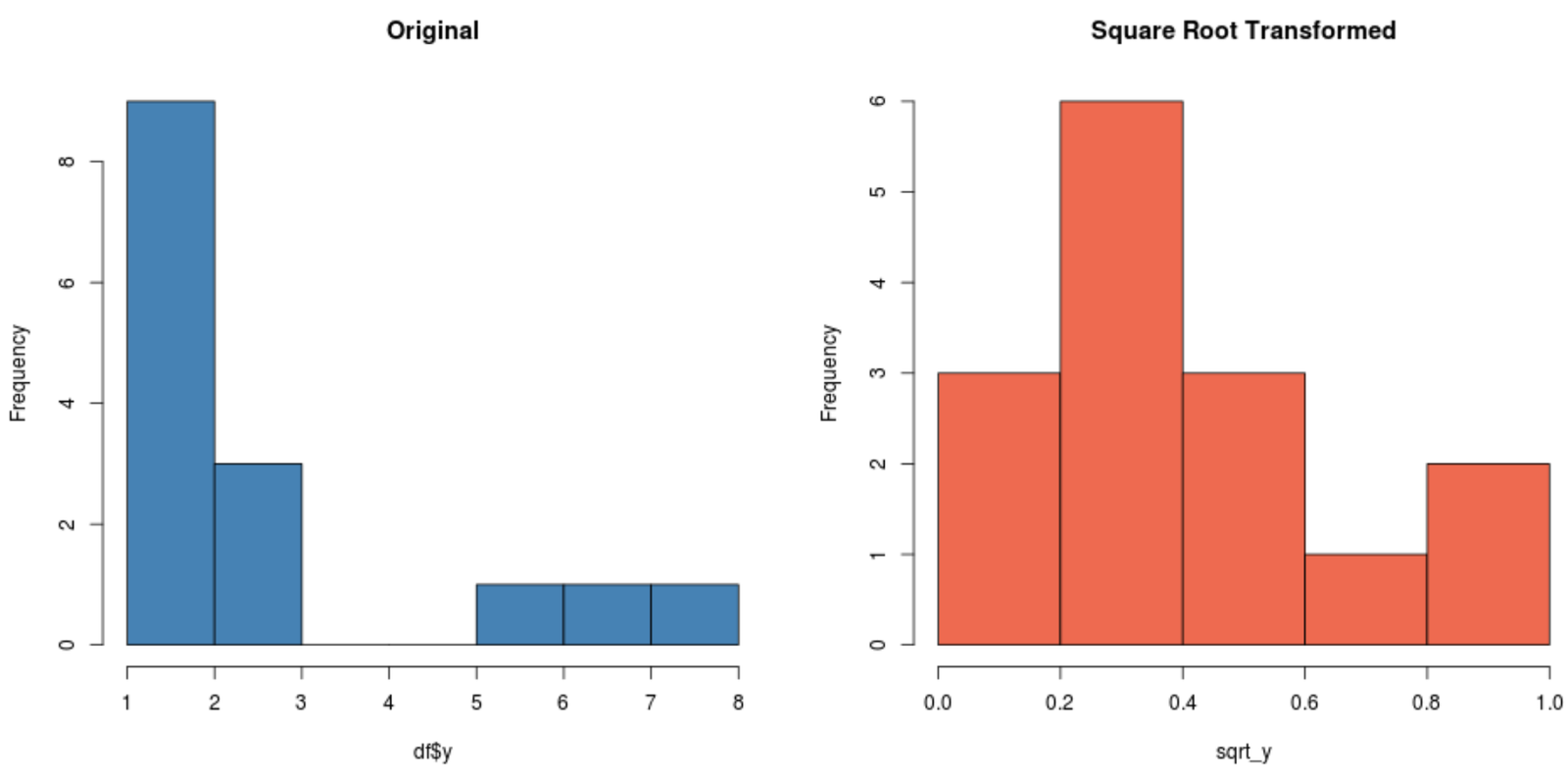
Notice how the square root-transformed distribution is much more normally distributed compared to the original distribution.
Cube Root Transformation in R
The following code shows how to perform a cube root transformation on a response variable:
#create data frame
df #perform square root transformation
cube_y
The following code shows how to create histograms to view the distribution of y before and after performing a square root transformation:
#create histogram for original distribution
hist(df$y, col='steelblue', main='Original')

#create histogram for square root-transformed distribution
hist(cube_y, col='coral2', main='Cube Root Transformed')
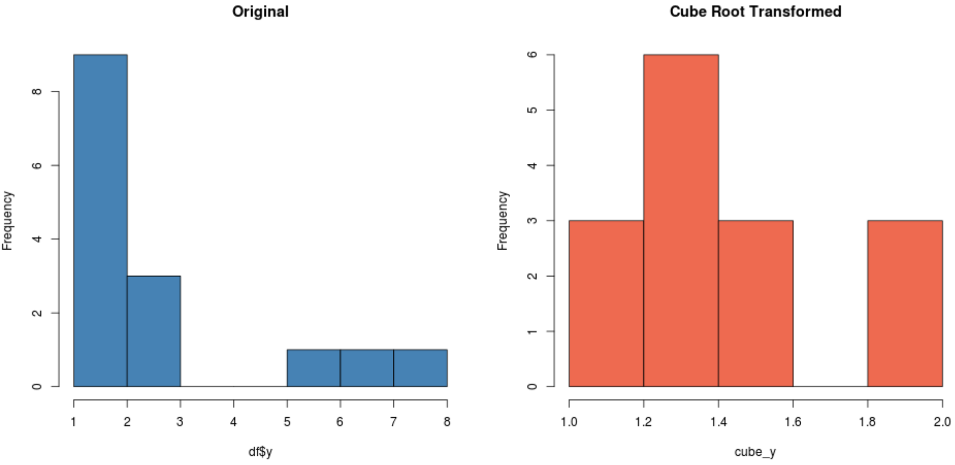
Depending on your dataset, one of these transformations may produce a new dataset that is more normally distributed than the others.