You can use the following basic formula to compare two lists in Excel using the VLOOKUP function:
=ISNA(VLOOKUP(A2,$C$2:$C$9,1,False))
Using the Conditional Formatting tool in Excel, we can use this formula to highlight every value in column A that does not belong to a range in column C.
The following example shows how to use this formula in practice.
Example: Compare Two Lists Using VLOOKUP
Suppose we have the following two datasets in Excel:
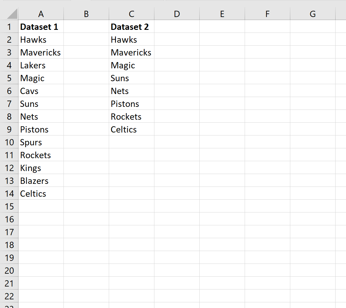
Suppose we’d like to identify the teams in Dataset 1 that are not in Dataset 2.
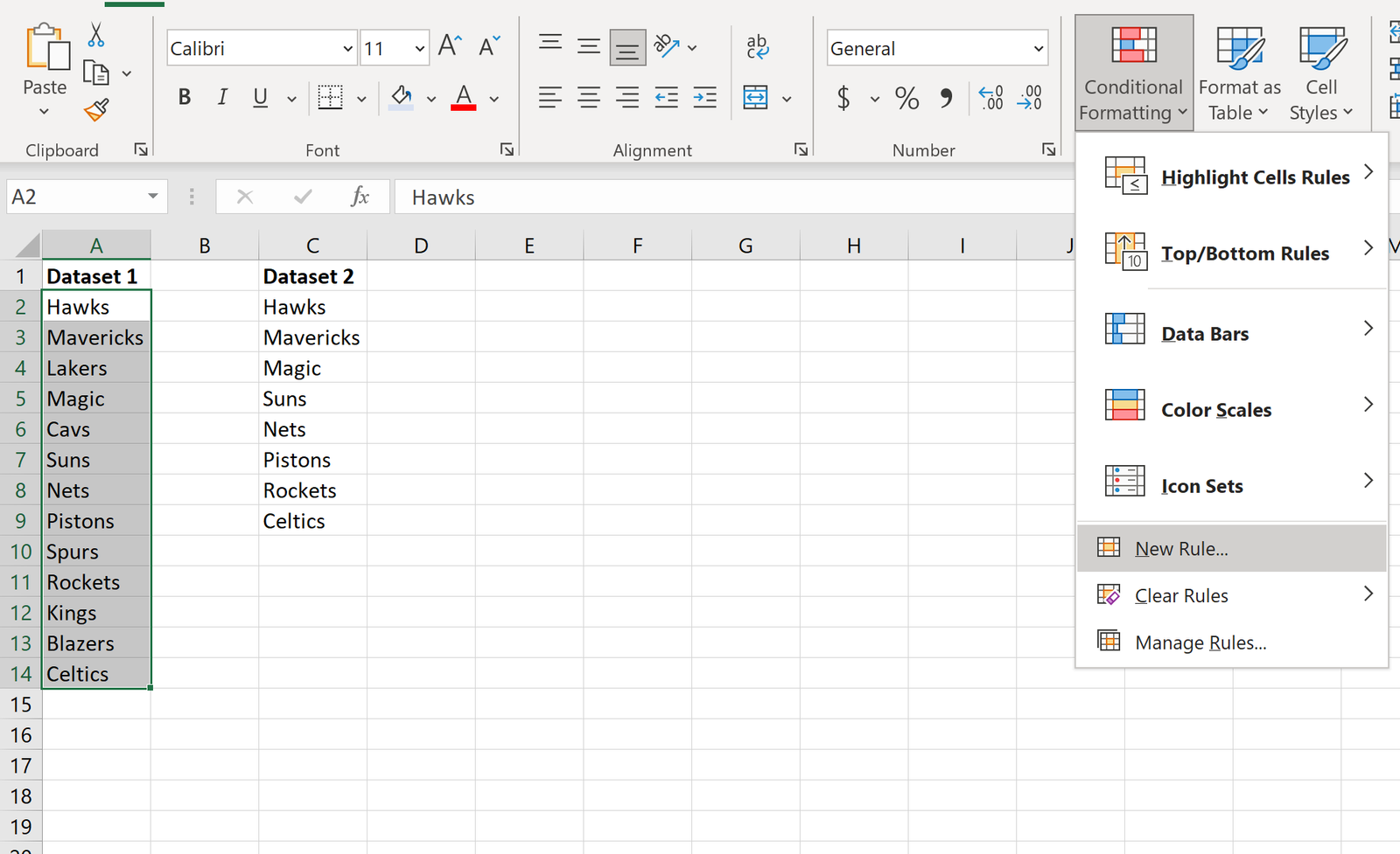
To do so, we can highlight every value in column A and then click the Conditional Formatting button on the Home tab along the top ribbon.
We can then click New Rule…
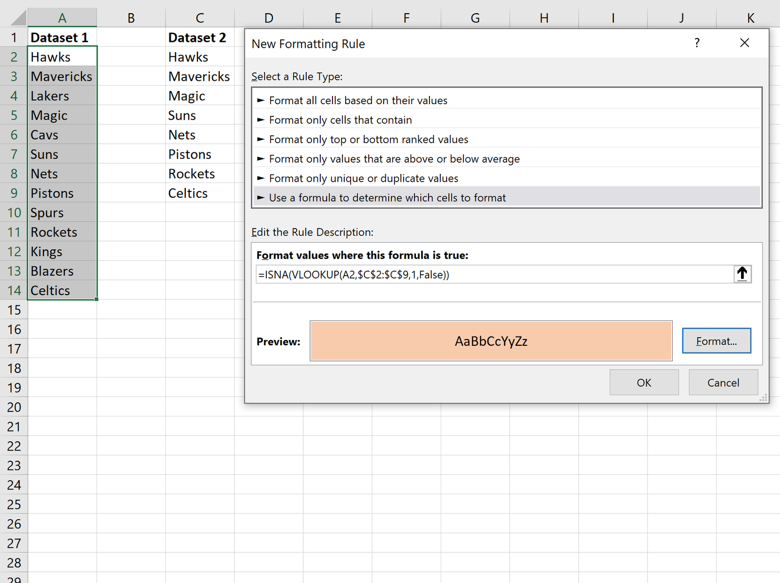
In the new window that appears, select the option that says Use a formula to determine which cells to format then type in the following formula:
=ISNA(VLOOKUP(A2,$C$2:$C$9,1,False))
Then click the Format button and choose a color to fill in values:
Once you click OK, every value in column A that does not appear in column C will be highlighted:

We can manually verify that a few of the values are highlighted correctly:
- Hawks appear in both Dataset 1 and Dataset 2, so it is not highlighted.
- Mavericks appear in both Dataset 1 and Dataset 2, so it is not highlighted.
- Lakers appear in Dataset 1 but not Dataset 2, so it is highlighted.
And so on.
Note that we chose to highlight values that did not belong to both datasets, but we could also apply a different styling such as bolded text, increased font size, a border around cells, etc.
Additional Resources
How to Compare Two Excel Sheets for Differences
How to Calculate the Difference Between Two Dates in Excel