A two-way ANOVA (“analysis of variance”) is used to determine whether or not there is a statistically significant difference between the means of three or more independent groups that have been split on two factors.
This tutorial explains how to perform a two-way ANOVA in Excel.
Example: Two Way ANOVA in Excel
A botanist wants to know whether or not plant growth is influenced by sunlight exposure and watering frequency. She plants 40 seeds and lets them grow for two months under different conditions for sunlight exposure and watering frequency. After two months, she records the height of each plant. The results are shown below:
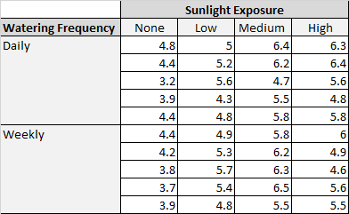
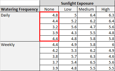
In the table above, we see that there were five plants grown under each combination of conditions. For example, there were five plants grown with daily watering and no sunlight and their heights after two months were 4.8 inches, 4.4 inches, 3.2 inches, 3.9 inches, and 4.4 inches:
We can use the following steps to perform a two-way ANOVA on this data:
Step 1: Select the Data Analysis Toolpak.
On the Data tab, click Data Analysis:
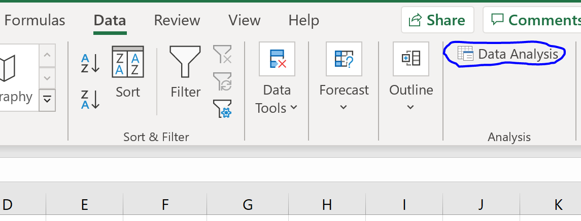
If you don’t see this as an option, you need to first load the free Data Analysis Toolpak.
2. Choose Anova: Two-Factor With Replication
Select the option that says Anova: Two-Factor With Replication, then click OK.
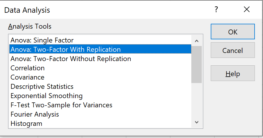
In this context, “replication” refers to having multiple observations in each group. For example, there were multiple plants that were grown with no sunlight exposure and daily watering. If instead we only grew one plant under each combination of conditions, we would use “without replication” but our sample size would be much smaller.
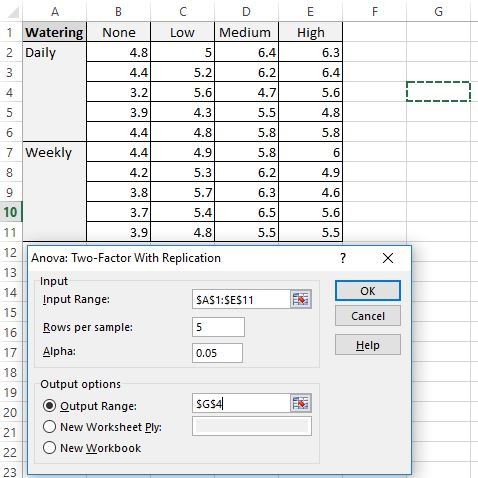
3. Fill in the necessary values.
Next, fill in the following values:
- Input Range: Select the cell range where our data lies, including the headings.
- Rows per sample: Type “5” because there are 5 plants in each sample.
- Alpha: Choose a significance level to use. We will choose 0.05.
- Output Range: Choose a cell where you would like the output of the two-way ANOVA to appear. We will choose cell $G$4.
Step 4: Interpret the output.
Once we click OK, the output of the two-way ANOVA will appear:

The first three tables show summary statistics for each group. For example:
- The average height of plants that were watered daily but given no sunlight was 4.14 inches.
- The average height of plants that were watered weekly and given low sunlight was 5.22 inches.
- The average height of all plants that were watered daily was 5.115 inches.
- The average height of all plants that were watered weekly was 5.15 inches.
- The average height of all plants that received high sunlight was 5.55 inches.
And so on.
The last table shows the result of the two-way ANOVA. We can observe the following:
- The p-value for the interaction between watering frequency and sunlight exposure was 0.310898. This is not statistically significant at alpha level 0.05.
- The p-value for watering frequency was 0.975975. This is not statistically significant at alpha level 0.05.
- The p-value for sunlight exposure was 3.9E-8 (0.000000039). This is statistically significant at alpha level 0.05.
These results indicate that sunlight exposure is the only factor that has a statistically significant effect on plant height. And because there is no interaction effect, the effect of sunlight exposure is consistent across each level of watering frequency. That is, whether a plant is watered daily or weekly has no impact on how sunlight exposure affects a plant.