The following step-by-step example shows how to create a pivot table from multiple sheets in Google Sheets.
Step 1: Enter the Data
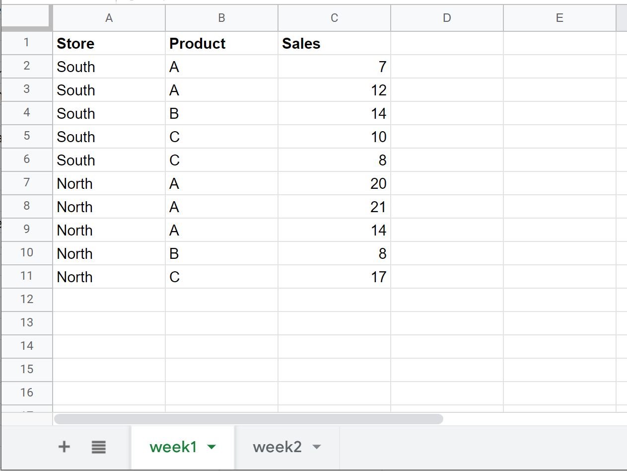
Suppose we have a spreadsheet with two sheets titled week1 and week2:
Week1:
Week2:

Suppose we would like to create a pivot table using data from both sheets.
Step 2: Consolidate Data into One Sheet
Before we can create a pivot table using both sheets, we must consolidate all of the data into one sheet.
We can use the following QUERY formula to do so:
=QUERY({week1!A1:C11;week2!A2:C11})
Here’s how to use this formula in practice:

Notice that the data from the week1 and week2 sheets are now consolidated into one sheet.
Step 3: Create the Pivot Table
To create the pivot table, we’ll highlight the values in the range A1:C21, then click the Insert tab and then click Pivot table.
We can then create the following pivot table:

The final pivot table includes data from both the week1 and week2 sheets.
Additional Resources
The following tutorials explain how to perform other common operations in Google Sheets:
Google Sheets: How to Sort a Pivot Table
Google Sheets: How to Add Calculated Field in Pivot Table
Google Sheets: Display Percentage of Total in Pivot Table