You can use the following basic syntax to use the IMPORTRANGE function in Google Sheets with specific conditions:
=QUERY(IMPORTRANGE("URL","Sheet1!A1:G9"),"where Col2='Spurs'")
This returns only the data in the range A1:G9 from the tab named Sheet1 within the Google Sheets spreadsheet with a specific URL where the second column has a value of Spurs.
The following example shows how to use this syntax in practice.
Example: Use IMPORTRANGE with Conditions
Suppose the data we’re interested in is located in a Google Sheets spreadsheet within a tab called stats at the following URL:

We can use the following syntax to return only the rows from this tab where the value in the second column is equal to Spurs:
=QUERY(IMPORTRANGE("1AdlE9V0aYMdrCmAGtvGXIEfo3szQ1tWRJ2HhJkUhg_4",
"stats!A1:C12"), "where Col2='Spurs'")
The following screenshot shows how to use this syntax in practice:
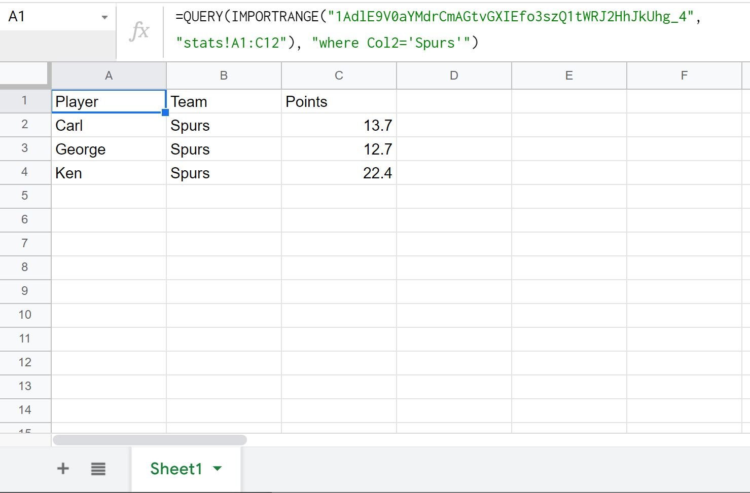
Notice that only the rows with the team name Spurs are returned.
You can also use the select statement to only return specific columns from the original spreadsheet.
For example, you can use the following syntax to return the values from only the Player and Points columns for the rows where the second column is equal to Spurs:
=QUERY(IMPORTRANGE("1AdlE9V0aYMdrCmAGtvGXIEfo3szQ1tWRJ2HhJkUhg_4",
"stats!A1:C12"), "select Col1, Col3 where Col2='Spurs'")
The following screenshot shows how to use this syntax in practice:
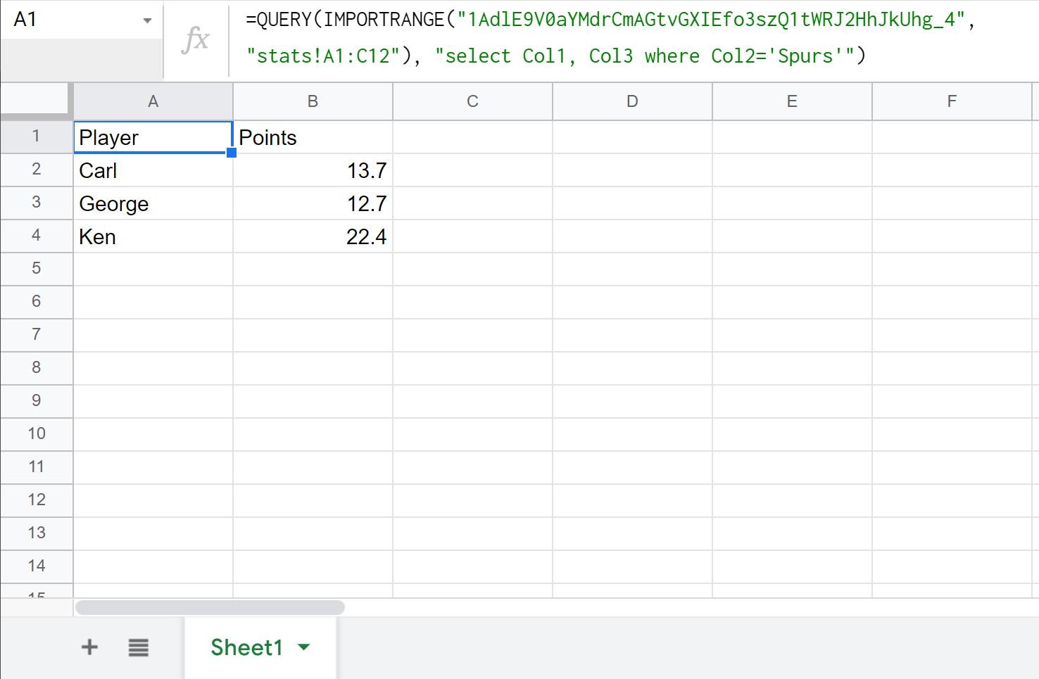
Notice that only the Player and Points columns are returned where the team name is equal to Spurs.
Additional Resources
The following tutorials explain how to perform other common tasks in Google Sheets:
Google Sheets: How to Query From Another Sheet
Google Sheets Query: How to Use Multiple Criteria in Query
Google Sheets Query: How to Return Only Unique Rows