You can use the following basic syntax to perform a VLOOKUP from another workbook in Google Sheets:
=VLOOKUP(A2, IMPORTRANGE("1AdlE5drC", "'sheet1'!$A$1:$B$11"), 2, 0)
This particular formula will look up the value in cell A2 of the current workbook in the range A1:B11 of a second workbook that has a spreadsheet key of 1AdlE5drC and return the corresponding value in the second column.
The following step-by-step example shows how to use this formula in practice.
Step 1: Enter Data into Both Workbooks
Suppose our current workbook contains the following data:

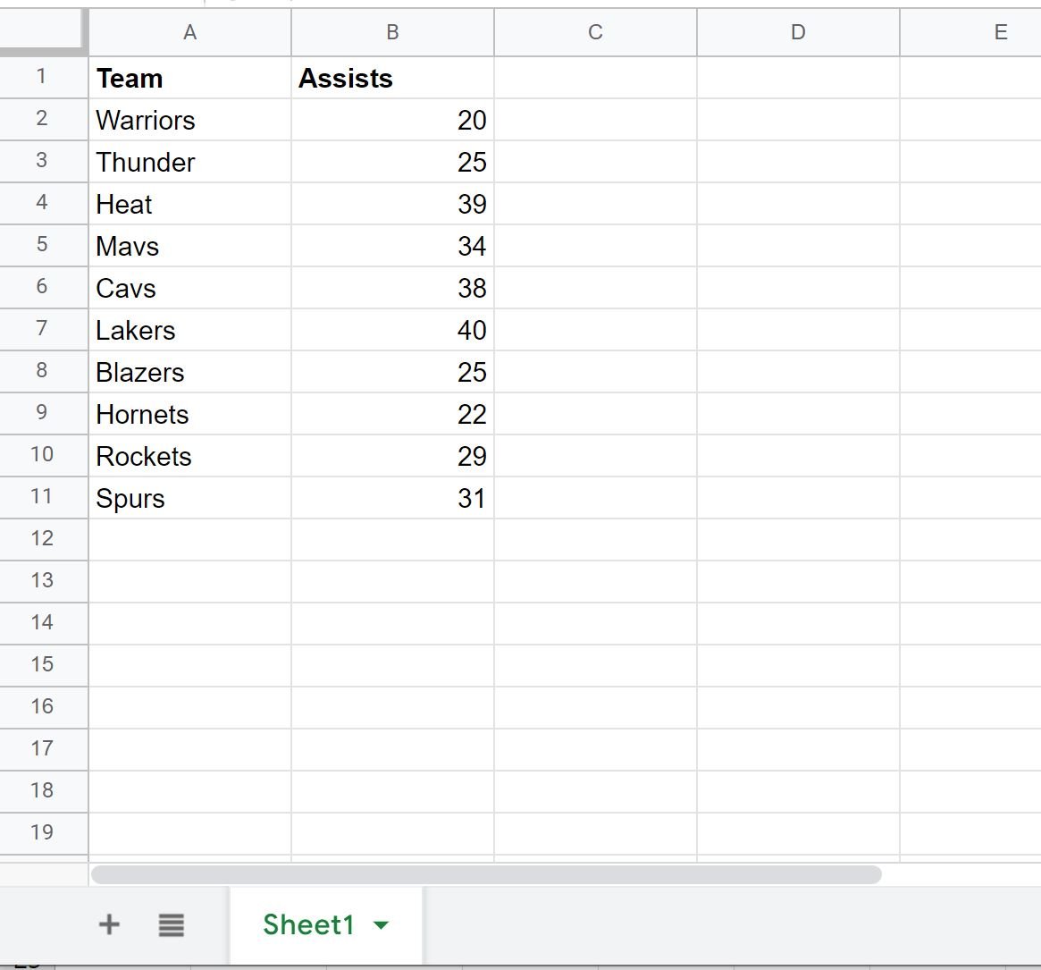
And suppose we have another workbook with the following data:
Step 2: Perform VLOOKUP Between Workbooks
Now suppose we would like to use a VLOOKUP in the first workbook to look up the team names in the second workbook and return the corresponding value in the Assists column.
Before we perform this VLOOKUP, we must find the spreadsheet key in the URL of the second workbook:

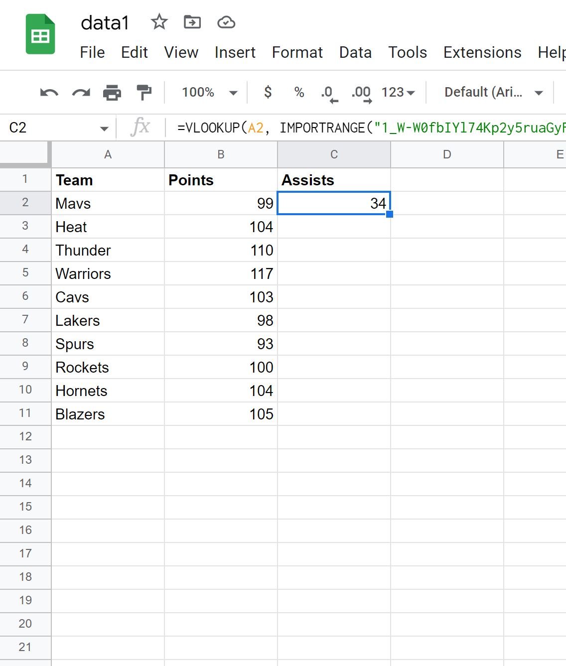
We can then type the following formula into cell C2 of the first workbook:
=VLOOKUP(A2, IMPORTRANGE("1_W-W0fbIYl74Kp2y5ruaGyFjWOskrcPBdQ6Vk_t_dRQ", "'sheet1'!$A$1:$B$11"), 2, 0)
Once we press Enter, the value in the Assists column from the second workbook that corresponds to the “Mavs” team will be shown:
We can then drag and fill this formula down to each remaining cell in column C to find the Assists values for each team:
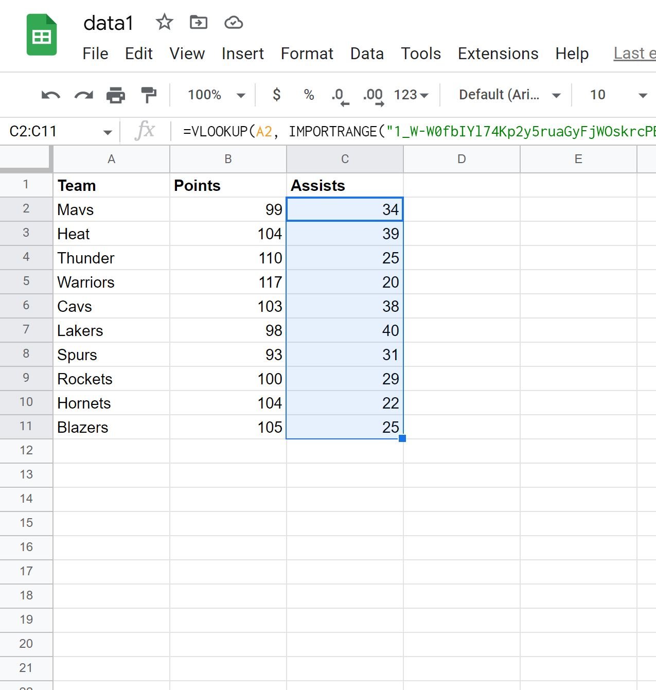
The values in the Assists column of the second workbook have now all been pulled into the first workbook.
Additional Resources
The following tutorials explain how to perform other common operations in Google Sheets:
Google Sheets: Use IMPORTRANGE with Multiple Sheets
Google Sheets: How to Use IMPORTRANGE with Conditions
Google Sheets: Use VLOOKUP with Multiple Criteria