The following step-by-step example shows how to highlight the top 10% of values in a column in Google Sheets.
Step 1: Enter the Data
First, let’s enter the following dataset into Google Sheets:

Step 2: Highlight Top 10% of Values
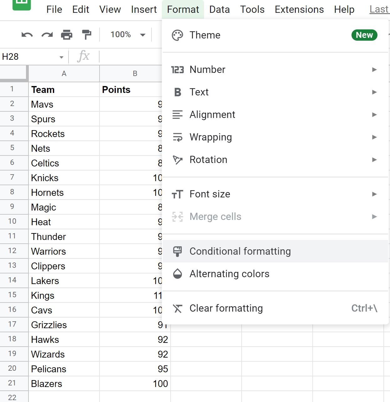
Next, click the Format tab and then click Conditional formatting:
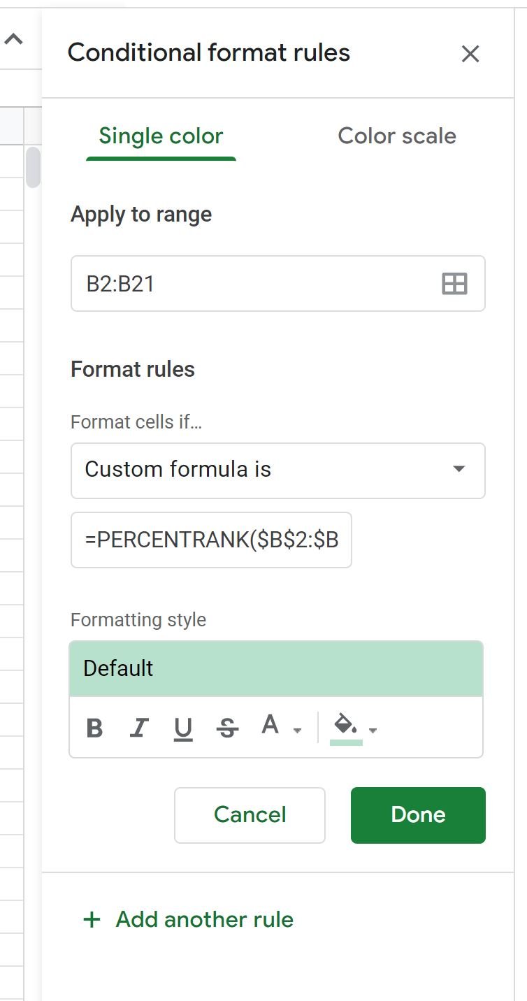
In the Conditional format rules panel that appears on the right side of the screen, type B2:B21 in the Apply to range box, then choose Custom formula is in the Format rules dropdown box, then type in the following formula:
=PERCENTRANK($B$2:$B$21,B2)>=90%
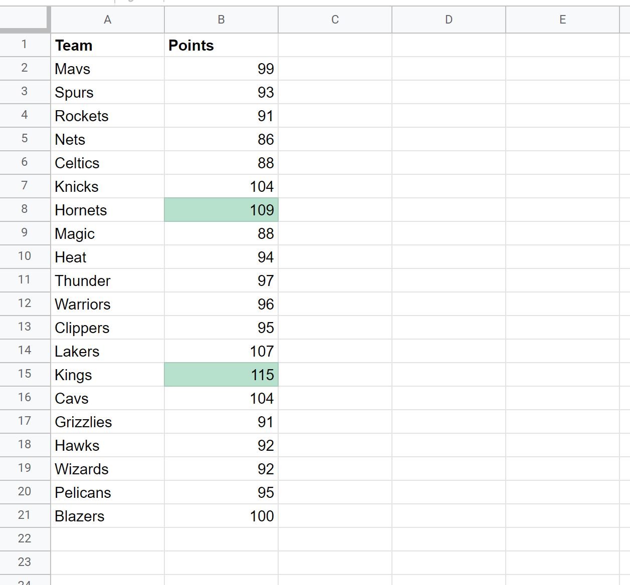
Once you click Done, the top 10% of values in the Points column will be highlighted:
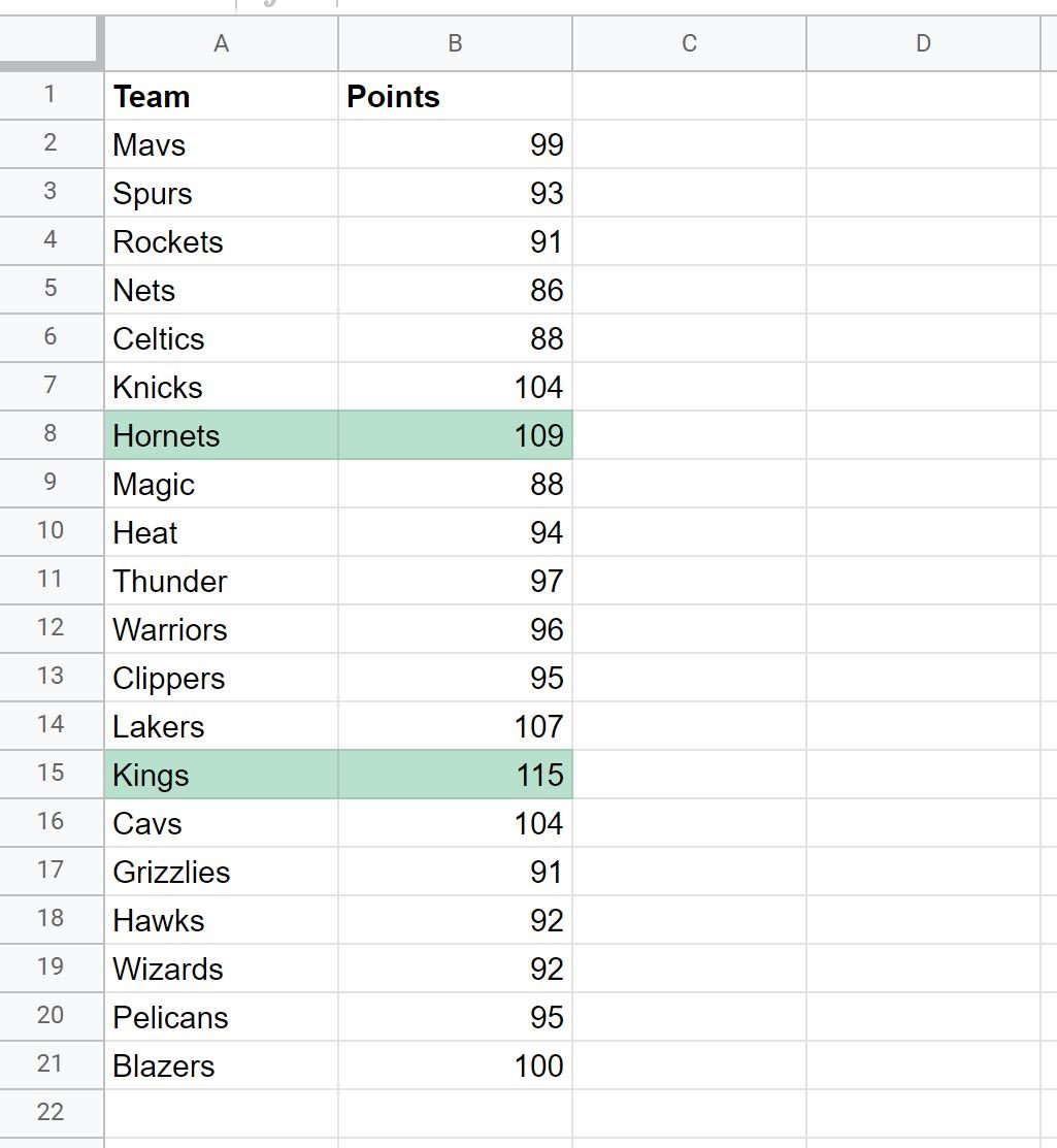
If you would like to highlight the entire row that contains the top 10% of values in the Points column, type A2:B21 in the Apply to range box, then choose Custom formula is in the Format rules dropdown box, then type in the following formula:
=PERCENTRANK($B$2:$B$21,$B2)>=90%
Once you click Done, the entire row that contains the top 10% of values in the Points column will be highlighted:
Additional Resources
The following tutorials explain how to perform other common tasks in Google Sheets:
How to Calculate Standard Deviation in Google Sheets
How to Calculate Descriptive Statistics in Google Sheets
How to Calculate the Interquartile Range in Google Sheets