You can use the MOD function in Google Sheets to calculate the remainder after a division operation.
This function uses the following basic syntax:
=MOD(dividend, divisor)
where:
- dividend: The number to be divided
- divisor: The number to divide by
The following examples show to use this function in different scenarios in Google Sheets.
Example 1: Using MOD Function with No Remainder
The following screenshot shows how to use the MOD function in a situation where there is no remainder:

From the output we can see that the remainder of 36 divided by 6 is zero.
This is because 6 divides into 36 exactly 6 times and no remainder is left.
Example 2: Using MOD Function with a Remainder
The following screenshot shows how to use the MOD function in a situation where there is a remainder:
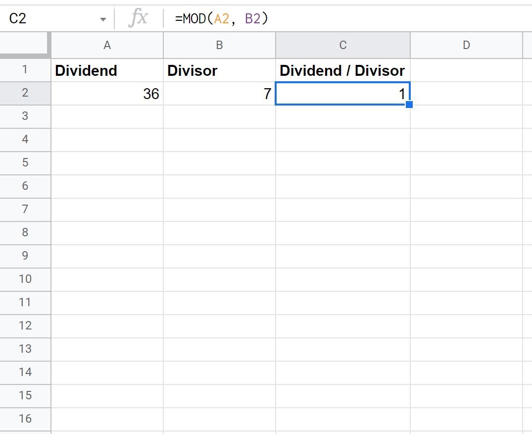
From the output we can see that the remainder of 36 divided by 7 is one.
This is because 7 divides into 36 a total of 5 times and a remainder of 1 is left.
Example 3: Using MOD Function when Dividing by Zero
The following screenshot shows the result of using the MOD function when we attempt to divide by zero:
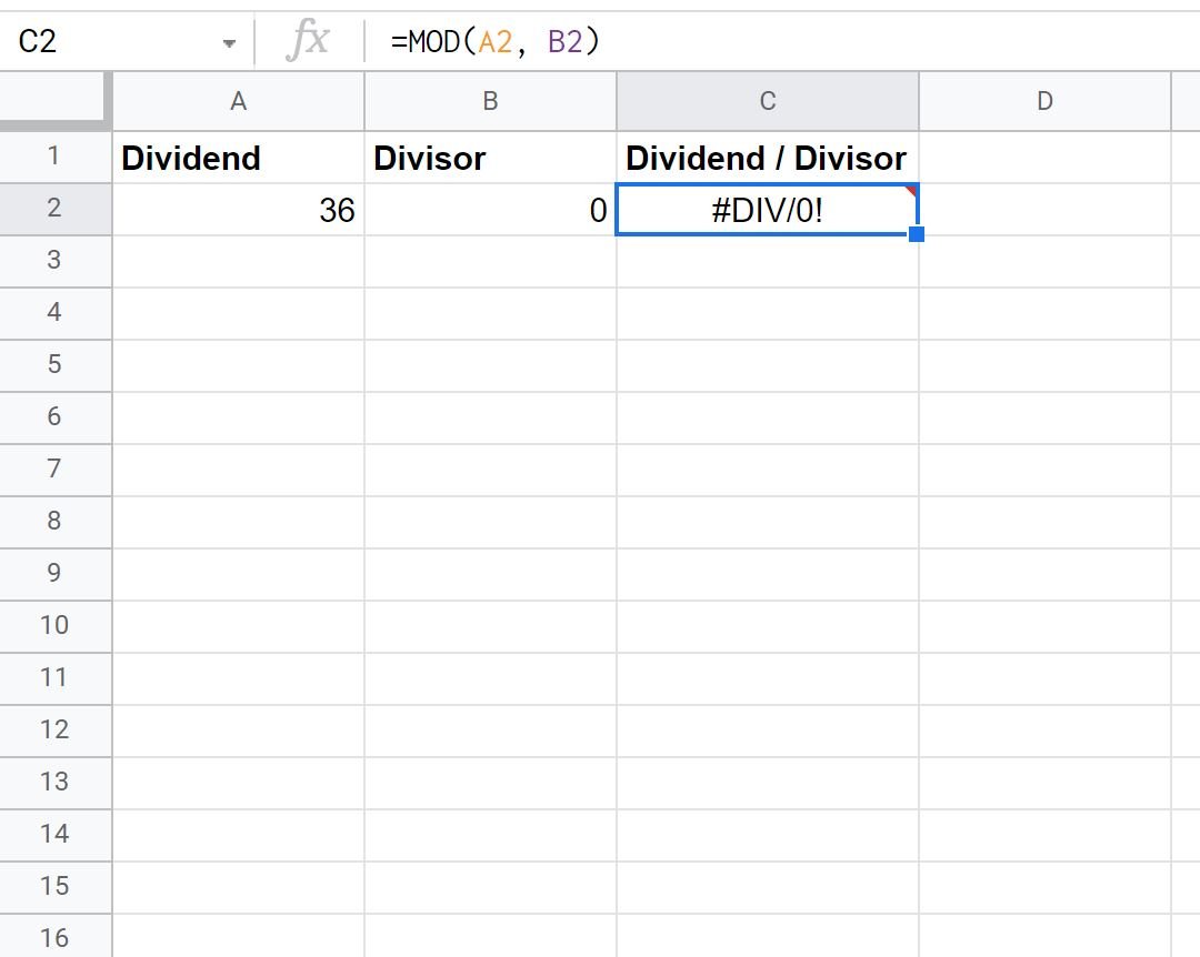
We receive a #DIV/0! error because it’s not possible to divide by zero.
If we’d like to suppress this error, we can instead use the following formula:
=IFERROR(MOD(A2, B2), "")
The following screenshot shows how to use this formula in practice:
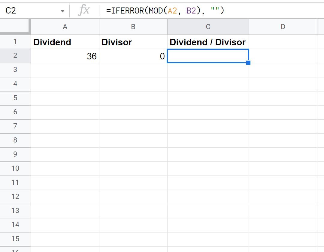
Since we attempted to divide by zero, the formula simply returned a blank value as a result.
Note: You can find the complete online documentation for the MOD function here.
Additional Resources
The following tutorials explain how to use other common functions in Google Sheets:
How to Use AVERAGEIFS Function in Google Sheets
How to Use ISERROR Function in Google Sheets
How to Ignore #N/A Values with Formulas in Google Sheets