Linear regression is used to find a line that best “fits” a dataset.
We often use three different sum of squares values to measure how well the regression line actually fits the data:
1. Sum of Squares Total (SST) – The sum of squared differences between individual data points (yi) and the mean of the response variable (y).
- SST = Σ(yi – y)2
2. Sum of Squares Regression (SSR) – The sum of squared differences between predicted data points (ŷi) and the mean of the response variable(y).
- SSR = Σ(ŷi – y)2
3. Sum of Squares Error (SSE) – The sum of squared differences between predicted data points (ŷi) and observed data points (yi).
- SSE = Σ(ŷi – yi)2
The following relationship exists between these three measures:
SST = SSR + SSE
Thus, if we know two of these measures then we can use some simple algebra to calculate the third.
SSR, SST & R-Squared
R-squared, sometimes referred to as the coefficient of determination, is a measure of how well a linear regression model fits a dataset. It represents the proportion of the variance in the response variable that can be explained by the predictor variable.
The value for R-squared can range from 0 to 1. A value of 0 indicates that the response variable cannot be explained by the predictor variable at all. A value of 1 indicates that the response variable can be perfectly explained without error by the predictor variable.
Using SSR and SST, we can calculate R-squared as:
R-squared = SSR / SST
For example, if the SSR for a given regression model is 137.5 and SST is 156 then we would calculate R-squared as:
R-squared = 137.5 / 156 = 0.8814
This tells us that 88.14% of the variation in the response variable can be explained by the predictor variable.
Calculate SST, SSR, SSE: Step-by-Step Example
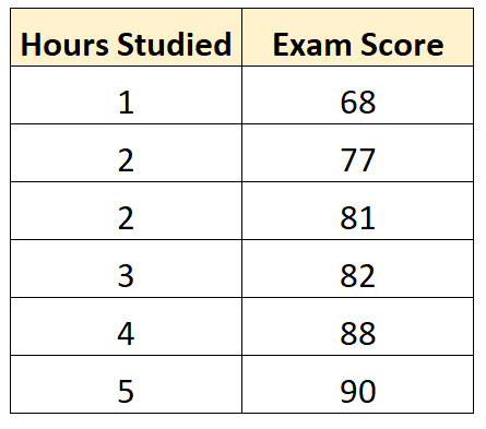
Suppose we have the following dataset that shows the number of hours studied by six different students along with their final exam scores:
Using some statistical software (like R, Excel, Python) or even by hand, we can find that the line of best fit is:
Score = 66.615 + 5.0769*(Hours)
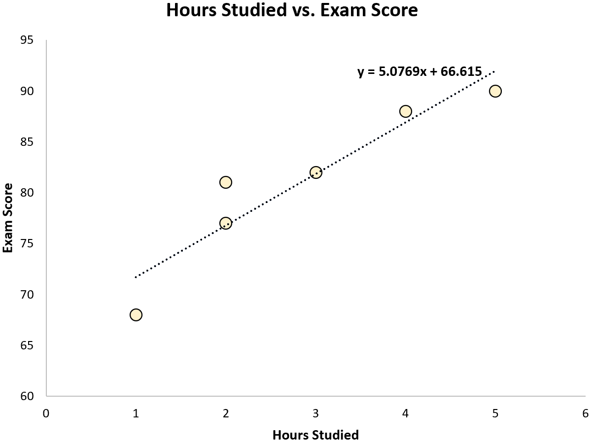
Once we know the line of best fit equation, we can use the following steps to calculate SST, SSR, and SSE:
Step 1: Calculate the mean of the response variable.
The mean of the response variable (y) turns out to be 81.
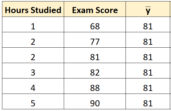
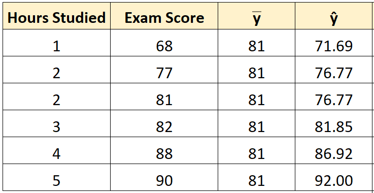
Step 2: Calculate the predicted value for each observation.
Next, we can use the line of best fit equation to calculate the predicted exam score () for each student.
For example, the predicted exam score for the student who studied one hours is:
Score = 66.615 + 5.0769*(1) = 71.69.
We can use the same approach to find the predicted score for each student:
Step 3: Calculate the sum of squares total (SST).
Next, we can calculate the sum of squares total.
For example, the sum of squares total for the first student is:
(yi – y)2 = (68 – 81)2 = 169.
We can use the same approach to find the sum of squares total for each student:

The sum of squares total turns out to be 316.
Step 4: Calculate the sum of squares regression (SSR).
Next, we can calculate the sum of squares regression.
For example, the sum of squares regression for the first student is:
(ŷi – y)2 = (71.69 – 81)2 = 86.64.
We can use the same approach to find the sum of squares regression for each student:
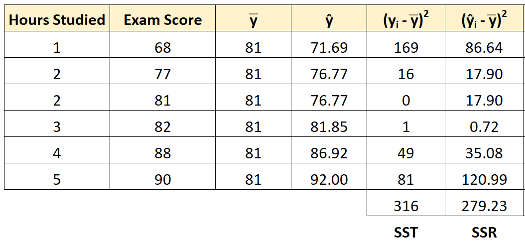
The sum of squares regression turns out to be 279.23.
Step 5: Calculate the sum of squares error (SSE).
Next, we can calculate the sum of squares error.
For example, the sum of squares error for the first student is:
(ŷi – yi)2 = (71.69 – 68)2 = 13.63.
We can use the same approach to find the sum of squares error for each student:
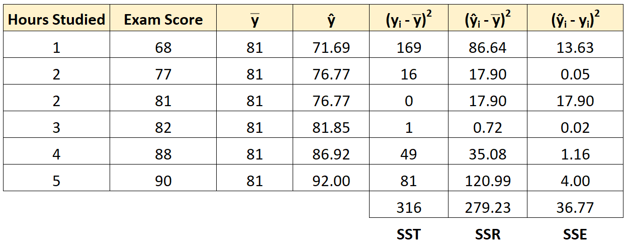
We can verify that SST = SSR + SSE
- SST = SSR + SSE
- 316 = 279.23 + 36.77
We can also calculate the R-squared of the regression model by using the following equation:
- R-squared = SSR / SST
- R-squared = 279.23 / 316
- R-squared = 0.8836
This tells us that 88.36% of the variation in exam scores can be explained by the number of hours studied.
Additional Resources
You can use the following calculators to automatically calculate SST, SSR, and SSE for any simple linear regression line: